Learning Networks

Below is a practical guide to the MLJ implementation of learning networks, which have been described more abstractly in the article:

Anthony D. Blaom and Sebastian J. Voller (2020): Flexible model composition in machine learning and its implementation in MLJ. Preprint, arXiv:2012.15505.

Learning networks, an advanced but powerful MLJ feature, are "blueprints" for combining models in flexible ways, beyond ordinary linear pipelines and simple model ensembles. They are simple transformations of your existing workflows which can be "exported" to define new, re-usable composite model types (models which typically have other models as hyperparameters).

Pipeline models (see Pipeline), and model stacks (see Stack) are both implemented internally as exported learning networks.

Learning networks by example

Learning networks are best explained by way of example.

Lazy computation

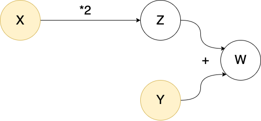
The core idea of a learning network is delayed or lazy computation. Instead of

X = 4
Y = 3
Z = 2*X
W = Y + Z
W

11

we can do

using MLJ

X = source(4)
Y = source(3)
Z = 2*X
W = Y + Z
W()

11

In the first computation X, Y, Z and W are all bound to ordinary data. In the second, they are bound to objects called nodes. The special nodes X and Y constitute "entry points" for data, and are called source nodes. As the terminology suggests, we can imagine these objects as part of a "network" (a directed acyclic graph) which can aid conceptualization (but is less useful in more complicated examples):

The origin of a node

The source nodes on which a given node depends are called the origins of the node:

os = origins(W)

2-element Vector{Source}:
 Source @437 ⏎ `Count`
 Source @853 ⏎ `Count`

X in os

true

Re-using a network

The advantage of lazy evaluation is that we can change data at a source node to repeat the calculation with new data. One way to do this (discouraged in practice) is to use rebind!:

Z()

8

rebind!(X, 6) # demonstration only!
Z()

12

However, if a node has a unique origin, then one instead calls the node on the new data one would like to rebind to that origin:

origins(Z)

1-element Vector{Source}:
 Source @853 ⏎ `Count`

Z(6)

12

Z(4)

8

This has the advantage that you don't need to locate the origin and rebind data directly, and the unique-origin restriction turns out to be sufficient for the applications to learning we have in mind.

Overloading functions for use on nodes

Several built-in function like * and + above are overloaded in MLJBase to work on nodes, as illustrated above. Others that work out-of-the-box include: MLJBase.matrix, MLJBase.table, vcat, hcat, mean, median, mode, first, last, as well as broadcasted versions of log, exp, mean, mode and median. A function like sqrt is not overloaded, so that Q = sqrt(Z) will throw an error. Instead, we do

Q = node(z->sqrt(z), Z)
Z()

12

Q()

3.4641016151377544

You can learn more about the node function under More on defining new nodes

A network that learns

To incorporate learning in a network of nodes MLJ:

• Allows binding of machines to nodes instead of data

• Generates "operation" nodes when calling an operation like predict or transform on a machine and node input data. Such nodes point to both a machine (storing learned parameters) and the node from which to fetch data for applying the operation (which, unlike the nodes seen so far, depend on learned parameters to generate output).

For an example of a learning network that actually learns, we first synthesize some training data X, y, and production data Xnew:

using MLJ
X, y = make_blobs(cluster_std=10.0, rng=123)  # `X` is a table, `y` a vector
Xnew, _ = make_blobs(3) # `Xnew` is a table with the same number of columns

We choose a model do some dimension reduction, and another to perform classification:

pca = (@load PCA pkg=MultivariateStats verbosity=0)()
tree = (@load DecisionTreeClassifier pkg=DecisionTree verbosity=0)()

To make our learning lazy, we wrap the training data as source nodes:

Xs = source(X)
ys = source(y)

And, finally, proceed as we would in an ordinary MLJ workflow, with the exception that there is no need to fit! our machines, as training will be carried out lazily later:

mach1 = machine(pca, Xs)
x = transform(mach1, Xs) # defines a new node because `Xs` is a node

mach2 = machine(tree, x, ys)
yhat = predict(mach2, x) # defines a new node because `x` is a node

Node @094 → DecisionTreeClassifier(…)
  args:
    1:	Node @751 → PCA(…)
  formula:
    predict(
      machine(DecisionTreeClassifier(max_depth = -1, …), …), 
      transform(
        machine(PCA(maxoutdim = 0, …), …), 
        Source @159))

Note that mach1 and mach2 are not themselves nodes. They point to the nodes they need to call to get training data and they are in turn pointed to by other nodes. In fact, an interesting implementation detail is that an "ordinary" machine is not actually bound directly to data, but bound to data wrapped in source nodes.

machine(pca, Xnew).args[1] # `Xnew` is ordinary data

Source @042 ⏎ `Table{AbstractVector{Continuous}}`

Before calling a node, we need to fit! the node, to trigger training of all the machines on which it depends:

julia> fit!(yhat)   # can include same keyword options for `fit!(::Machine, ...)`[ Info: Training machine(PCA(maxoutdim = 0, …), …).
[ Info: Training machine(DecisionTreeClassifier(max_depth = -1, …), …).
Node @094 → DecisionTreeClassifier(…)
  args:
    1:	Node @751 → PCA(…)
  formula:
    predict(
      machine(DecisionTreeClassifier(max_depth = -1, …), …),
      transform(
        machine(PCA(maxoutdim = 0, …), …),
        Source @159))
julia> yhat()[1:2]  # or `yhat(rows=2)`2-element UnivariateFiniteVector{Multiclass{3}, Int64, UInt32, Float64}:
 UnivariateFinite{Multiclass{3}}(1=>1.0, 2=>0.0, 3=>0.0)
 UnivariateFinite{Multiclass{3}}(1=>1.0, 2=>0.0, 3=>0.0)

This last represents the prediction on the training data, because that's what resides at our source nodes. However, yhat has the unique origin X (because "training edges" in the complete associated directed graph are excluded for this purpose). We can therefore call yhat on our production data to get the corresponding predictions:

yhat(Xnew)

3-element UnivariateFiniteVector{Multiclass{3}, Int64, UInt32, Float64}:
 UnivariateFinite{Multiclass{3}}(1=>0.0, 2=>0.0, 3=>1.0)
 UnivariateFinite{Multiclass{3}}(1=>0.0, 2=>0.0, 3=>1.0)
 UnivariateFinite{Multiclass{3}}(1=>1.0, 2=>0.0, 3=>0.0)

Training is smart, in the sense that mutating a hyper-parameter of some component model does not force retraining of upstream machines:

julia> tree.max_depth = 11
julia> fit!(yhat)[ Info: Not retraining machine(PCA(maxoutdim = 0, …), …). Use `force=true` to force.
[ Info: Updating machine(DecisionTreeClassifier(max_depth = 1, …), …).
Node @094 → DecisionTreeClassifier(…)
  args:
    1:	Node @751 → PCA(…)
  formula:
    predict(
      machine(DecisionTreeClassifier(max_depth = 1, …), …),
      transform(
        machine(PCA(maxoutdim = 0, …), …),
        Source @159))
julia> yhat(Xnew)3-element UnivariateFiniteVector{Multiclass{3}, Int64, UInt32, Float64}:
 UnivariateFinite{Multiclass{3}}(1=>0.357, 2=>0.4, 3=>0.243)
 UnivariateFinite{Multiclass{3}}(1=>0.357, 2=>0.4, 3=>0.243)
 UnivariateFinite{Multiclass{3}}(1=>0.357, 2=>0.4, 3=>0.243)

Multithreaded training

A more complicated learning network may contain machines that can be trained in parallel. In that case, a call like the following may speed up training:

tree.max_depth=2
fit!(yhat, acceleration=CPUThreads())

[ Info: Not retraining machine(PCA(maxoutdim = 0, …), …). Use `force=true` to force.
[ Info: Updating machine(DecisionTreeClassifier(max_depth = 2, …), …).

Currently, only CPU1() (default) and CPUThreads() are supported here.

Exporting a learning network as a new model type

Once a learning network has been tested, typically on some small dummy data set, it is ready to be exported as a new, stand-alone, re-usable model type (unattached to any data). We demonstrate the process by way of examples of increasing complexity:

• Example A - Mini-pipeline
• More on replacing models with symbols
• Example B - Multiple operations: transform and inverse transform
• Example C - Blending predictions and exposing internal network state in reports
• Example D - Multiple nodes pointing to the same machine
• Example E - Coupling component model hyper-parameters
• More on defining new nodes
• Example F - Wrapping a model in a data-dependent tuning strategy

Example A - Mini-pipeline

First we export the simple learning network defined above. (This is for illustration purposes; in practice using the Pipeline syntax model1 |> model2 syntax is more convenient.)

Step 1 - Define a new model struct

We need a type with two fields, one for the preprocessor (pca in the network above) and one for the classifier (tree in the network above).

The DecisionTreeClassifier type of tree has supertype Probabilistic, because it makes probabilistic predictions, and we assume any other classifier we want to swap out will be the same.

supertype(typeof(tree))

Probabilistic

In particular, our composite model will also need Probabilistic as supertype. In fact, we must give it the intermediate supertype ProbabilisticNetworkComposite <: Probabilistic, so that we additionally flag it as an exported learning network model type:

mutable struct CompositeA <: ProbabilisticNetworkComposite
    preprocessor
    classifier
end

The common alternatives are DeterministicNetworkComposite and UnsupervisedNetworkComposite. But all options can be viewed as follows:

using MLJBase
NetworkComposite

NetworkComposite (alias for Union{AnnotatorNetworkComposite, DeterministicNetworkComposite, DeterministicSupervisedDetectorNetworkComposite, DeterministicUnsupervisedDetectorNetworkComposite, IntervalNetworkComposite, JointProbabilisticNetworkComposite, ProbabilisticNetworkComposite, ProbabilisticSetNetworkComposite, ProbabilisticSupervisedDetectorNetworkComposite, ProbabilisticUnsupervisedDetectorNetworkComposite, StaticNetworkComposite, SupervisedAnnotatorNetworkComposite, SupervisedDetectorNetworkComposite, SupervisedNetworkComposite, UnsupervisedAnnotatorNetworkComposite, UnsupervisedDetectorNetworkComposite, UnsupervisedNetworkComposite})

We next make our learning network model-generic by substituting each model instance with the corresponding symbol representing a property (field) of the new model struct:

mach1 = machine(:preprocessor, Xs)   # <---- `pca` swapped out for `:preprocessor`
x = transform(mach1, Xs)
mach2 = machine(:classifier, x, ys)  # <---- `tree` swapped out for `:classifier`
yhat = predict(mach2, x)

Node @413 → :classifier
  args:
    1:	Node @455 → :preprocessor
  formula:
    predict(
      machine(:classifier, …), 
      transform(
        machine(:preprocessor, …), 
        Source @159))

Incidentally, this network can be used as before except we must provide an instance of CompositeA in our fit! calls, to indicate what actual models the symbols are being substituted with:

composite_a = CompositeA(pca, ConstantClassifier())
fit!(yhat, composite=composite_a)
yhat(Xnew)

3-element UnivariateFiniteVector{Multiclass{3}, Int64, UInt32, Float64}:
 UnivariateFinite{Multiclass{3}}(1=>0.33, 2=>0.33, 3=>0.34)
 UnivariateFinite{Multiclass{3}}(1=>0.33, 2=>0.33, 3=>0.34)
 UnivariateFinite{Multiclass{3}}(1=>0.33, 2=>0.33, 3=>0.34)

In this case :preprocessor is being substituted by pca, and :classifier by ConstantClassifier() for training.

Step 2 - Wrap the learning network in prefit

Literally copy and paste the learning network above into the definition of a method called prefit, as shown below (if you have implemented your own MLJ model, you will notice this has the same signature as MLJModelInterface.fit):

import MLJBase
function MLJBase.prefit(composite::CompositeA, verbosity, X, y)

        # the learning network from above:
        Xs = source(X)
        ys = source(y)
        mach1 = machine(:preprocessor, Xs)
        x = transform(mach1, Xs)
        mach2 = machine(:classifier, x, ys)
        yhat = predict(mach2, x)

        verbosity > 0 && @info "I'm a noisy fellow!"

        # return "learning network interface":
        return (; predict=yhat)
end

That's it.

Generally, prefit always returns a learning network interface; see MLJBase.prefit for what this means in general. In this example, the interface dictates that calling predict(mach, Xnew) on a machine mach bound to some instance of CompositeA should internally call yhat(Xnew).

Here's our new composite model type CompositeA in action, combining standardization with KNN classification:

using MLJ
X, y = @load_iris

knn = (@load KNNClassifier pkg=NearestNeighborModels verbosity=0)()
composite_a = CompositeA(Standardizer(), knn)

CompositeA(
  preprocessor = Standardizer(
        features = Symbol[], 
        ignore = false, 
        ordered_factor = false, 
        count = false), 
  classifier = KNNClassifier(
        K = 5, 
        algorithm = :kdtree, 
        metric = Distances.Euclidean(0.0), 
        leafsize = 10, 
        reorder = true, 
        weights = NearestNeighborModels.Uniform()))

mach = machine(composite_a, X, y) |> fit!
predict(mach, X)[1:2]

2-element UnivariateFiniteVector{Multiclass{3}, String, UInt32, Float64}:
 UnivariateFinite{Multiclass{3}}(setosa=>1.0, versicolor=>0.0, virginica=>0.0)
 UnivariateFinite{Multiclass{3}}(setosa=>1.0, versicolor=>0.0, virginica=>0.0)

report(mach).preprocessor

(features_fit = [:sepal_length, :petal_width, :petal_length, :sepal_width],)

fitted_params(mach).classifier

(tree = NearestNeighbors.KDTree{StaticArraysCore.SVector{4, Float64}, Distances.Euclidean, Float64, StaticArraysCore.SVector{4, Float64}}
  Number of points: 150
  Dimensions: 4
  Metric: Distances.Euclidean(0.0)
  Reordered: true,)

More on replacing models with symbols

Only the first argument model in some expression machine(model, ...) can be replaced with a symbol. These replacements function as hooks for exposing reports and fitted parameters of component models in the report and fitted parameters of the composite model, but these replacements are not absolutely necessary. For example, instead of the line mach1 = machine(:preprocessor, Xs) in the prefit definition, we can do mach1 = machine(composite.preprocessor, Xs). However, report and fittted_params will not include items for the :preprocessor component model in that case.

If a component model is not explicitly bound to data in a machine (for example, because it is first wrapped in TunedModel) then there are ways to explicitly expose associated fitted parameters or report items. See Example F below.

Example B - Multiple operations: transform and inverse transform

Here's a second mini-pipeline example composing two transformers which both implement inverse transform. We show how to implement an inverse_transform for the composite model too.

Step 1 - Define a new model struct

using MLJ
import MLJBase

mutable struct CompositeB <: DeterministicNetworkComposite
    transformer1
    transformer2
end

Step 2 - Wrap the learning network in prefit

function MLJBase.prefit(composite::CompositeB, verbosity, X)
    Xs = source(X)

    mach1 = machine(:transformer1, Xs)
    X1 = transform(mach1, Xs)
    mach2 = machine(:transformer2, X1)
    X2 = transform(mach2, X1)

    W1 = inverse_transform(mach2, Xs)
    W2 = inverse_transform(mach1, W1)

    # the learning network interface:
    return (; transform=X2, inverse_transform=W2)
end

Here's a demonstration:

X = rand(100)

composite_b = CompositeB(UnivariateBoxCoxTransformer(), Standardizer())
mach = machine(composite_b, X) |> fit!
W =  transform(mach, X)
@assert inverse_transform(mach, W) ≈ X

Example C - Blending predictions and exposing internal network state in reports

The code below defines a new composite model type CompositeC that predicts by taking the weighted average of two regressors, and additionally exposes, in the model's report, a measure of disagreement between the two models at time of training. In addition to the two regressors, the new model has two other fields:

• mix, controlling the weighting

• acceleration, for the mode of acceleration for training the model (e.g., CPUThreads()).

Step 1 - Define a new model struct

using MLJ
import MLJBase

mutable struct CompositeC <: DeterministicNetworkComposite
    regressor1
    regressor2
    mix::Float64
    acceleration
end

Step 2 - Wrap the learning network in prefit

function MLJBase.prefit(composite::CompositeC, verbosity, X, y)

    Xs = source(X)
    ys = source(y)

    mach1 = machine(:regressor1, Xs, ys)
    mach2 = machine(:regressor2, Xs, ys)

    yhat1 = predict(mach1, Xs)
    yhat2 = predict(mach2, Xs)

    # node to return disagreement between the regressor predictions:
    disagreement = node((y1, y2) -> l2(y1, y2) |> mean, yhat1, yhat2)

    # get the weighted average the predictions of the regressors:
    λ = composite.mix
    yhat = (1 - λ)*yhat1 + λ*yhat2

    # the learning network interface:
    return (
        predict = yhat,
        report= (; training_disagreement=disagreement),
        acceleration = composite.acceleration,
    )

end

Here's a demonstration:

X, y = make_regression() # a table and a vector

knn = (@load KNNRegressor pkg=NearestNeighborModels verbosity=0)()
tree =  (@load DecisionTreeRegressor pkg=DecisionTree verbosity=0)()
composite_c = CompositeC(knn, tree, 0.2, CPUThreads())
mach = machine(composite_c, X, y) |> fit!
Xnew, _ = make_regression(3)
predict(mach, Xnew)

3-element Vector{Float64}:
 -0.7029764091986238
 -0.7553231974592023
 -0.6270125193923791

report(mach)

(regressor2 = (features = [:x1, :x2],),
 training_disagreement = 0.0027608495393292233,
 predict = (regressor2 = (features = [:x1, :x2],),),)

Example D - Multiple nodes pointing to the same machine

When incorporating learned target transformations (such as a standardization) in supervised learning, it is desirable to apply the inverse transformation to predictions, to return them to the original scale. This means re-using learned parameters from an earlier part of your workflow. This poses no problem here, as the next example demonstrates.

The model type CompositeD defined below applies a preprocessing transformation to input data X (e.g., standardization), learns a transformation for the target y (e.g., an optimal Box-Cox transformation), predicts new target values using a regressor (e.g., Ridge regression), and then inverse-transforms those predictions to restore them to the original scale. (This represents a model we could alternatively build using the TransformedTargetModel wrapper and a Pipeline.)

Step 1 - Define a new model struct

using MLJ
import MLJBase

mutable struct CompositeD <: DeterministicNetworkComposite
    preprocessor
    target_transformer
    regressor
    acceleration
end

Step 2 - Wrap the learning network in prefit

Notice that both of the nodes z and yhat in the wrapped learning network point to the same machine (learned parameters) mach2.

function MLJBase.prefit(composite::CompositeD, verbosity, X, y)

    Xs = source(X)
    ys = source(y)

    mach1 = machine(:preprocessor, Xs)
    W = transform(mach1, Xs)

    mach2 = machine(:target_transformer, ys)
    z = transform(mach2, ys)

    mach3 =machine(:regressor, W, z)
    zhat = predict(mach3, W)

    yhat = inverse_transform(mach2, zhat)

    # the learning network interface:
    return (
        predict = yhat,
        acceleration = composite.acceleration,
    )

end

The flow of information in the wrapped learning network is visualized below.

Here's an application of our new composite to the Boston dataset:

X, y = @load_boston

stand = Standardizer()
box = UnivariateBoxCoxTransformer()
ridge = (@load RidgeRegressor pkg=MultivariateStats verbosity=0)(lambda=92)
composite_d = CompositeD(stand, box, ridge, CPU1())
evaluate(composite_d, X, y, resampling=CV(nfolds=5), measure=l2, verbosity=0)

PerformanceEvaluation object with these fields:
  model, measure, operation, measurement, per_fold,
  per_observation, fitted_params_per_fold,
  report_per_fold, train_test_rows, resampling, repeats
Extract:
┌──────────┬───────────┬─────────────┬─────────┬────────────────────────────────
│ measure  │ operation │ measurement │ 1.96*SE │ per_fold                      ⋯
├──────────┼───────────┼─────────────┼─────────┼────────────────────────────────
│ LPLoss(  │ predict   │ 27.9        │ 20.0    │ [9.26, 23.1, 33.6, 60.4, 13.4 ⋯
│   p = 2) │           │             │         │                               ⋯
└──────────┴───────────┴─────────────┴─────────┴────────────────────────────────
                                                                1 column omitted

Example E - Coupling component model hyper-parameters

The composite model in this example combines a clustering model used to reduce the dimension of the feature space (KMeans or KMedoids from Clustering.jl) with ridge regression, but has the following "coupling" of the hyperparameters: The amount of ridge regularization depends on the number of specified clusters k, with less regularization for a greater number of clusters. It includes a user-specified coupling coefficient c, and exposes the solver hyper-parameter of the ridge regressor. (Neither the clusterer nor ridge regressor are themselves hyperparameters of the composite.)

Step 1 - Define a new model struct

using MLJ
import MLJBase

mutable struct CompositeE <: DeterministicNetworkComposite
        clusterer     # `:kmeans` or `:kmedoids`
        k::Int        # number of clusters
        solver        # a ridge regression parameter we want to expose
        c::Float64    # a "coupling" coefficient
end

Step 2 - Wrap the learning network in prefit

RidgeRegressor = @load RidgeRegressor pkg=MLJLinearModels verbosity=0
KMeans   = @load KMeans pkg=Clustering verbosity=0
KMedoids = @load KMedoids pkg=Clustering verbosity=0

function MLJBase.prefit(composite::CompositeE, verbosity, X, y)

        Xs = source(X)
        ys = source(y)

        k = composite.k
        solver = composite.solver
        c = composite.c

        clusterer = composite.clusterer == :kmeans ? KMeans(; k) : KMedoids(; k)
        mach1 = machine(clusterer, Xs)
        Xsmall = transform(mach1, Xs)

        # the coupling - ridge regularization depends on the number of
        # clusters `k` and the coupling coefficient `c`:
        lambda = exp(-c/k)

        ridge = RidgeRegressor(; lambda, solver)
        mach2 = machine(ridge, Xsmall, ys)
        yhat = predict(mach2, Xsmall)

        return (predict=yhat,)
end

Here's an application to the Boston dataset in which we optimize the coupling coefficient (see Tuning Models for more on hyper-parameter optimization):

X, y = @load_boston # a table and a vector

composite_e = CompositeE(:kmeans, 3, nothing, 0.5)
r = range(composite_e, :c, lower = -2, upper=2, scale=x->10^x)
tuned_composite_e = TunedModel(
    composite_e,
    range=r,
    tuning=RandomSearch(rng=123),
    measure=l2,
    resampling=CV(nfolds=6),
    n=100,
)
mach = machine(tuned_composite_e, X, y) |> fit!
report(mach).best_model

CompositeE(
  clusterer = :kmeans, 
  k = 3, 
  solver = nothing, 
  c = 0.14720178188876742)

More on defining new nodes

Overloading ordinary functions for nodes has already been discussed above. Here's another example:

divide(x, y) = x/y

X = source(2)
Y = source(3)

Z = node(divide, X, Y)

This means Z() returns divide(X(), Y()), which is divide(2, 3) in this case:

Z()

0.6666666666666666

We cannot call Z with arguments (e.g., Z(2)) because it does not have a unique origin.

In all the node examples so far, the first argument of node is a function, and all other arguments are nodes - one node for each argument of the function. A node constructed in this way is called a static node. A dynamic node, which directly depends on the outcome of a training event, is constructed by giving a machine as the second argument, to be passed as the first argument of the function in a node call. For example, we can do

Xs = source(rand(4))
mach = machine(Standardizer(), Xs)
N = node(transform, mach, Xs) |> fit!

[ Info: Training machine(Standardizer(features = Symbol[], …), …).

Then N has the following calling properties:

• N() returns transform(mach, Xs())
• N(Xnew) returns transform(mach, Xs(Xnew)); here Xs(Xnew) is just Xnew because Xs is just a source node.)

N()

4-element Vector{Float64}:
  0.3097277718673464
 -1.4244083620630208
  0.20105872362694022
  0.9136218665687336

N(rand(2))

2-element Vector{Float64}:
  0.6707127594719003
 -0.8770485483419167

In fact, this is precisely how the transform method is internally overloaded to work, when called with a node argument (to return a node instead of data). That is, internally there exists code that amounts to the definition

transform(mach, X::AbstractNode) = node(transform, mach, X)

Here AbstractNode is the common super-type of Node and Source.

It sometimes useful to create dynamic nodes with no node arguments, as in

Xs = source(rand(10))
mach = machine(Standardizer(), Xs)
N = node(fitted_params, mach) |> fit!
N()

(mean = 0.46023189664355446,
 std = 0.3287060402337959,)

Static nodes can have also have zero node arguments. These may be viewed as "constant" nodes:

N = Node(()-> 42)
N()

42

Example F below demonstrates the use of static and dynamic nodes. For more details, see the node docstring.

There is also an experimental macro @node. If Z is an AbstractNode (Z = source(16), say) then instead of

Q = node(z->sqrt(z), Z)

one can do

Q = @node sqrt(Z)

(so that Q() == 4). Here's a more complicated application of @node to row-shuffle a table:

using Random
X = (x1 = [1, 2, 3, 4, 5],
         x2 = [:one, :two, :three, :four, :five])
rows(X) = 1:nrows(X)

Xs = source(X)
rs  = @node rows(Xs)
W = @node selectrows(Xs, @node shuffle(rs))

julia> W()
(x1 = [5, 1, 3, 2, 4],
 x2 = Symbol[:five, :one, :three, :two, :four],)

Important. An argument not in global scope is assumed by @node to be a node or source.

Example F - Wrapping a model in a data-dependent tuning strategy

When the regularization parameter of a Lasso model is optimized, one commonly searches over a parameter range depending on properties of the training data. Indeed, Lasso (and, more generally, elastic net) implementations commonly provide a method to carry out this data-dependent optimization automatically, using cross-validation. The following example shows how to transform the LassoRegressor model type from MLJLinearModels.jl into a self-tuning model type LassoCVRegressor using the commonly implemented data-dependent tuning strategy. A new dimensionless hyperparameter epsilon controls the lower bound on the parameter range.

Step 1 - Define a new model struct

using MLJ
import MLJBase

mutable struct LassoCVRegressor <: DeterministicNetworkComposite
    lasso              # the atomic lasso model (`lasso.lambda` is ignored)
    epsilon::Float64   # controls lower bound of `lasso.lambda` in tuning
    resampling         # resampling strategy for optimization of `lambda`
end

# keyword constructor for convenience:
LassoRegressor = @load LassoRegressor pkg=MLJLinearModels verbosity=0
LassoCVRegressor(;
    lasso=LassoRegressor(),
    epsilon=0.001,
    resampling=CV(nfolds=6),
) = LassoCVRegressor(
    lasso,
    epsilon,
    resampling,
)

Step 2 - Wrap the learning network in prefit

In this case, there is no model -> :symbol replacement that makes sense here, because the model is getting wrapped by TunedModel before being bound to nodes in a machine. However, we can expose the the learned lasso coefs and intercept using fitted parameter nodes; and expose the optimal lambda, and range searched, using report nodes (as previously demonstrated in Example C).

function MLJBase.prefit(composite::LassoCVRegressor, verbosity, X, y)

    λ_max = maximum(abs.(MLJ.matrix(X)'y))

    Xs = source(X)
    ys = source(y)

    r = range(
        composite.lasso,
        :lambda,
        lower=composite.epsilon*λ_max,
        upper=λ_max,
        scale=:log10,
    )

    lambda_range = node(()->r)  # a "constant" report node

    tuned_lasso = TunedModel(
        composite.lasso,
        tuning=Grid(shuffle=false),
        range = r,
        measure = l2,
        resampling=composite.resampling,
    )
    mach = machine(tuned_lasso, Xs, ys)

    R = node(report, mach)                                 # `R()` returns `report(mach)`
    lambda = node(r -> r.best_model.lambda, R)             # a report node

    F = node(fitted_params, mach)             # `F()` returns `fitted_params(mach)`
    coefs = node(f->f.best_fitted_params.coefs, F)         # a fitted params node
    intercept = node(f->f.best_fitted_params.intercept, F) # a fitted params node

    yhat = predict(mach, Xs)

    return (
        predict=yhat,
        fitted_params=(; coefs, intercept),
        report=(; lambda, lambda_range),
   )

end

Here's a demonstration:

X, _ = make_regression(1000, 3, rng=123)
y = X.x2 - X.x2 + 0.005*X.x3 + 0.05*rand(1000)
lasso_cv = LassoCVRegressor(epsilon=1e-5)
mach = machine(lasso_cv, X, y) |> fit!
report(mach)

(lambda = 0.00042546886155141466,
 lambda_range = NumericRange(3.294e-5 ≤ lambda ≤ 3.294; origin=1.647, unit=1.647; on log10 scale),)

fitted_params(mach)

(coefs = [:x1 => 0.0, :x2 => -0.0, :x3 => 0.004147704827722941],
 intercept = 0.02486029602840344,)

The learning network API

Two new julia types are part of learning networks: Source and Node, which share a common abstract supertype AbstractNode.

Formally, a learning network defines two labeled directed acyclic graphs (DAG's) whose nodes are Node or Source objects, and whose labels are Machine objects. We obtain the first DAG from directed edges of the form $N1 -> N2$ whenever $N1$ is an argument of $N2$ (see below). Only this DAG is relevant when calling a node, as discussed in the examples above and below. To form the second DAG (relevant when calling or calling fit! on a node) one adds edges for which $N1$ is training argument of the machine which labels $N1$. We call the second, larger DAG, the completed learning network (but note only edges of the smaller network are explicitly drawn in diagrams, for simplicity).

Source nodes

Only source nodes can reference concrete data. A Source object has a single field, data.

Source

Xs = source(X=nothing)

Xs() = X
Xs(rows=r) = selectrows(X, r)  # eg, X[r,:] for a DataFrame
Xs(Xnew) = Xnew

rebind!(s, X)

sources(N::AbstractNode)

origins(N)

Nodes

Node{T<:Union{Machine,Nothing}}

J = node(f, mach::Machine, args...)

J() = f(mach, args[1](), args[2](), ..., args[n]())
J(rows=r) = f(mach, args[1](rows=r), args[2](rows=r), ..., args[n](rows=r))
J(X) = f(mach, args[1](X), args[2](X), ..., args[n](X))

predict(mach, X::AbsractNode, y::AbstractNode)
predict_mean(mach, X::AbstractNode, y::AbstractNode)
predict_median(mach, X::AbstractNode, y::AbstractNode)
predict_mode(mach, X::AbstractNode, y::AbstractNode)
transform(mach, X::AbstractNode)
inverse_transform(mach, X::AbstractNode)

@node f(...)

X = source(π)
W = @node sin(X)
julia> W()
0

X = source(1:10)
Y = @node selectrows(X, 3:4)
julia> Y()
3:4

julia> Y(["one", "two", "three", "four"])
2-element Array{Symbol,1}:
 "three"
 "four"

X1 = source(4)
X2 = source(5)
add(a, b, c) = a + b + c
N = @node add(X1, 1, X2)
julia> N()
10

MLJBase.prefit(model, verbosity, data...)

 (predict=yhat,)
 (transform=Xsmall, acceleration=CPUThreads())
 (predict=yhat, transform=W, report=(loss=loss_node,))

 (k1=n1, k2=n2, ...)

See more on fitting nodes at fit! and fit_only!.