Common MLJ Workflows
Data ingestion
import RDatasets
channing = RDatasets.dataset("boot", "channing")

julia> first(channing, 4)
4×5 DataFrame
 Row │ Sex   Entry  Exit   Time   Cens
     │ Cat…  Int32  Int32  Int32  Int32
─────┼──────────────────────────────────
   1 │ Male    782    909    127      1
   2 │ Male   1020   1128    108      1
   3 │ Male    856    969    113      1
   4 │ Male    915    957     42      1
Inspecting metadata, including column scientific types:
schema(channing)┌───────┬───────────────┬──────────────────────────────────┐
│ names │ scitypes │ types │
├───────┼───────────────┼──────────────────────────────────┤
│ Sex │ Multiclass{2} │ CategoricalValue{String, UInt32} │
│ Entry │ Count │ Int64 │
│ Exit │ Count │ Int64 │
│ Time │ Count │ Int64 │
│ Cens │ Count │ Int64 │
└───────┴───────────────┴──────────────────────────────────┘
Horizontally splitting data and shuffling rows.
Here y is the :Exit column and X everything else:
y, X = unpack(channing, ==(:Exit), rng=123);Here y is the :Exit column and X everything else except :Time:
y, X =  unpack(channing,
               ==(:Exit),
               !=(:Time);
               rng=123);
scitype(y)
AbstractVector{Count} (alias for AbstractArray{Count, 1})schema(X)┌───────┬───────────────┬──────────────────────────────────┐
│ names │ scitypes │ types │
├───────┼───────────────┼──────────────────────────────────┤
│ Sex │ Multiclass{2} │ CategoricalValue{String, UInt32} │
│ Entry │ Count │ Int64 │
│ Cens │ Count │ Int64 │
└───────┴───────────────┴──────────────────────────────────┘
Fixing wrong scientific types in X:
X = coerce(X, :Exit=>Continuous, :Entry=>Continuous, :Cens=>Multiclass)
schema(X)
┌───────┬─────────────────┬──────────────────────────────────┐
│ names │ scitypes │ types │
├───────┼─────────────────┼──────────────────────────────────┤
│ Sex │ Multiclass{2} │ CategoricalValue{String, UInt32} │
│ Entry │ Continuous │ Float64 │
│ Cens │ Multiclass{462} │ CategoricalValue{Int64, UInt32} │
└───────┴─────────────────┴──────────────────────────────────┘
Loading a built-in supervised dataset:
table = load_iris();
schema(table)
┌──────────────┬───────────────┬──────────────────────────────────┐
│ names │ scitypes │ types │
├──────────────┼───────────────┼──────────────────────────────────┤
│ sepal_length │ Continuous │ Float64 │
│ sepal_width │ Continuous │ Float64 │
│ petal_length │ Continuous │ Float64 │
│ petal_width │ Continuous │ Float64 │
│ target │ Multiclass{3} │ CategoricalValue{String, UInt32} │
└──────────────┴───────────────┴──────────────────────────────────┘
Loading a built-in data set already split into X and y:
X, y = @load_iris;
selectrows(X, 1:4) # selectrows works whenever `Tables.istable(X)==true`.
(sepal_length = [5.1, 4.9, 4.7, 4.6],
sepal_width = [3.5, 3.0, 3.2, 3.1],
petal_length = [1.4, 1.4, 1.3, 1.5],
petal_width = [0.2, 0.2, 0.2, 0.2],)y[1:4]4-element CategoricalArray{String,1,UInt32}:
"setosa"
"setosa"
"setosa"
"setosa"Splitting data vertically after row shuffling:
channing_train, channing_test = partition(channing, 0.6, rng=123);Or, if already horizontally split:
(Xtrain, Xtest), (ytrain, ytest) = partition((X, y), 0.6, multi=true, rng=123)(((sepal_length = [6.7, 5.7, 7.2, 4.4, 5.6, 6.5, 4.4, 6.1, 5.4, 4.9 … 6.4, 5.5, 5.4, 4.8, 6.5, 4.9, 6.5, 6.7, 5.6, 6.4], sepal_width = [3.3, 2.8, 3.0, 2.9, 2.5, 3.0, 3.0, 2.9, 3.9, 2.5 … 3.1, 2.3, 3.7, 3.1, 3.0, 2.4, 2.8, 3.3, 2.9, 2.8], petal_length = [5.7, 4.1, 5.8, 1.4, 3.9, 5.2, 1.3, 4.7, 1.7, 4.5 … 5.5, 4.0, 1.5, 1.6, 5.5, 3.3, 4.6, 5.7, 3.6, 5.6], petal_width = [2.1, 1.3, 1.6, 0.2, 1.1, 2.0, 0.2, 1.4, 0.4, 1.7 … 1.8, 1.3, 0.2, 0.2, 1.8, 1.0, 1.5, 2.5, 1.3, 2.2]), (sepal_length = [6.0, 5.8, 6.7, 5.1, 5.0, 6.3, 5.7, 6.4, 6.1, 5.0 … 6.4, 6.8, 6.9, 6.1, 6.7, 5.0, 7.6, 6.3, 5.1, 5.0], sepal_width = [2.7, 2.6, 3.0, 3.8, 3.4, 2.8, 2.5, 3.2, 2.8, 3.5 … 2.7, 3.2, 3.1, 2.8, 2.5, 3.5, 3.0, 2.5, 3.8, 3.6], petal_length = [5.1, 4.0, 5.2, 1.9, 1.5, 5.1, 5.0, 4.5, 4.7, 1.6 … 5.3, 5.9, 5.4, 4.0, 5.8, 1.3, 6.6, 5.0, 1.6, 1.4], petal_width = [1.6, 1.2, 2.3, 0.4, 0.2, 1.5, 2.0, 1.5, 1.2, 0.6 … 1.9, 2.3, 2.1, 1.3, 1.8, 0.3, 2.1, 1.9, 0.2, 0.2])), (CategoricalValue{String, UInt32}["virginica", "versicolor", "virginica", "setosa", "versicolor", "virginica", "setosa", "versicolor", "setosa", "virginica" … "virginica", "versicolor", "setosa", "setosa", "virginica", "versicolor", "versicolor", "virginica", "versicolor", "virginica"], CategoricalValue{String, UInt32}["versicolor", "versicolor", "virginica", "setosa", "setosa", "virginica", "virginica", "versicolor", "versicolor", "setosa" … "virginica", "virginica", "virginica", "versicolor", "virginica", "setosa", "virginica", "virginica", "setosa", "setosa"]))Model Search
Reference: Model Search
Searching for a supervised model:
X, y = @load_boston
ms = models(matching(X, y))
69-element Vector{NamedTuple{(:name, :package_name, :is_supervised, :abstract_type, :deep_properties, :docstring, :fit_data_scitype, :human_name, :hyperparameter_ranges, :hyperparameter_types, :hyperparameters, :implemented_methods, :inverse_transform_scitype, :is_pure_julia, :is_wrapper, :iteration_parameter, :load_path, :package_license, :package_url, :package_uuid, :predict_scitype, :prediction_type, :reporting_operations, :reports_feature_importances, :supports_class_weights, :supports_online, :supports_training_losses, :supports_weights, :transform_scitype, :input_scitype, :target_scitype, :output_scitype)}}:
(name = ARDRegressor, package_name = MLJScikitLearnInterface, ... )
(name = AdaBoostRegressor, package_name = MLJScikitLearnInterface, ... )
(name = BaggingRegressor, package_name = MLJScikitLearnInterface, ... )
(name = BayesianRidgeRegressor, package_name = MLJScikitLearnInterface, ... )
(name = CatBoostRegressor, package_name = CatBoost, ... )
(name = ConstantRegressor, package_name = MLJModels, ... )
(name = DecisionTreeRegressor, package_name = BetaML, ... )
(name = DecisionTreeRegressor, package_name = DecisionTree, ... )
(name = DeterministicConstantRegressor, package_name = MLJModels, ... )
(name = DummyRegressor, package_name = MLJScikitLearnInterface, ... )
⋮
(name = SGDRegressor, package_name = MLJScikitLearnInterface, ... )
(name = SRRegressor, package_name = SymbolicRegression, ... )
(name = SVMLinearRegressor, package_name = MLJScikitLearnInterface, ... )
(name = SVMNuRegressor, package_name = MLJScikitLearnInterface, ... )
(name = SVMRegressor, package_name = MLJScikitLearnInterface, ... )
(name = StableForestRegressor, package_name = SIRUS, ... )
(name = StableRulesRegressor, package_name = SIRUS, ... )
(name = TheilSenRegressor, package_name = MLJScikitLearnInterface, ... )
(name = XGBoostRegressor, package_name = XGBoost, ... )ms[6](name = "ConstantRegressor",
package_name = "MLJModels",
is_supervised = true,
abstract_type = Probabilistic,
deep_properties = (),
docstring = "```\nConstantRegressor\n```\n\nThis \"dummy\" probabilis...",
fit_data_scitype = Tuple{Table, AbstractVector{Continuous}},
human_name = "constant regressor",
hyperparameter_ranges = (nothing,),
hyperparameter_types = ("Type{D} where D<:Distributions.Sampleable",),
hyperparameters = (:distribution_type,),
implemented_methods = [:fitted_params, :predict],
inverse_transform_scitype = Unknown,
is_pure_julia = true,
is_wrapper = false,
iteration_parameter = nothing,
load_path = "MLJModels.ConstantRegressor",
package_license = "MIT",
package_url = "https://github.com/alan-turing-institute/MLJModels.jl",
package_uuid = "d491faf4-2d78-11e9-2867-c94bc002c0b7",
predict_scitype = AbstractVector{ScientificTypesBase.Density{Continuous}},
prediction_type = :probabilistic,
reporting_operations = (),
reports_feature_importances = false,
supports_class_weights = false,
supports_online = false,
supports_training_losses = false,
supports_weights = false,
transform_scitype = Unknown,
input_scitype = Table,
target_scitype = AbstractVector{Continuous},
output_scitype = Unknown)models("Tree");28-element Vector{NamedTuple{(:name, :package_name, :is_supervised, :abstract_type, :deep_properties, :docstring, :fit_data_scitype, :human_name, :hyperparameter_ranges, :hyperparameter_types, :hyperparameters, :implemented_methods, :inverse_transform_scitype, :is_pure_julia, :is_wrapper, :iteration_parameter, :load_path, :package_license, :package_url, :package_uuid, :predict_scitype, :prediction_type, :reporting_operations, :reports_feature_importances, :supports_class_weights, :supports_online, :supports_training_losses, :supports_weights, :transform_scitype, :input_scitype, :target_scitype, :output_scitype)}}:
(name = ABODDetector, package_name = OutlierDetectionNeighbors, ... )
(name = AdaBoostStumpClassifier, package_name = DecisionTree, ... )
(name = COFDetector, package_name = OutlierDetectionNeighbors, ... )
(name = DNNDetector, package_name = OutlierDetectionNeighbors, ... )
(name = DecisionTreeClassifier, package_name = BetaML, ... )
(name = DecisionTreeClassifier, package_name = DecisionTree, ... )
(name = DecisionTreeRegressor, package_name = BetaML, ... )
(name = DecisionTreeRegressor, package_name = DecisionTree, ... )
(name = EvoTreeClassifier, package_name = EvoTrees, ... )
(name = EvoTreeCount, package_name = EvoTrees, ... )
⋮
(name = LOFDetector, package_name = OutlierDetectionNeighbors, ... )
(name = MultitargetKNNClassifier, package_name = NearestNeighborModels, ... )
(name = MultitargetKNNRegressor, package_name = NearestNeighborModels, ... )
(name = OneRuleClassifier, package_name = OneRule, ... )
(name = RandomForestClassifier, package_name = BetaML, ... )
(name = RandomForestClassifier, package_name = DecisionTree, ... )
(name = RandomForestRegressor, package_name = BetaML, ... )
(name = RandomForestRegressor, package_name = DecisionTree, ... )
(name = SMOTENC, package_name = Imbalance, ... )A more refined search:
models() do model
    matching(model, X, y) &&
    model.prediction_type == :deterministic &&
    model.is_pure_julia
end;
Searching for an unsupervised model:
models(matching(X))63-element Vector{NamedTuple{(:name, :package_name, :is_supervised, :abstract_type, :deep_properties, :docstring, :fit_data_scitype, :human_name, :hyperparameter_ranges, :hyperparameter_types, :hyperparameters, :implemented_methods, :inverse_transform_scitype, :is_pure_julia, :is_wrapper, :iteration_parameter, :load_path, :package_license, :package_url, :package_uuid, :predict_scitype, :prediction_type, :reporting_operations, :reports_feature_importances, :supports_class_weights, :supports_online, :supports_training_losses, :supports_weights, :transform_scitype, :input_scitype, :target_scitype, :output_scitype)}}:
(name = ABODDetector, package_name = OutlierDetectionNeighbors, ... )
(name = ABODDetector, package_name = OutlierDetectionPython, ... )
(name = AffinityPropagation, package_name = MLJScikitLearnInterface, ... )
(name = AgglomerativeClustering, package_name = MLJScikitLearnInterface, ... )
(name = AutoEncoder, package_name = BetaML, ... )
(name = Birch, package_name = MLJScikitLearnInterface, ... )
(name = BisectingKMeans, package_name = MLJScikitLearnInterface, ... )
(name = CBLOFDetector, package_name = OutlierDetectionPython, ... )
(name = CDDetector, package_name = OutlierDetectionPython, ... )
(name = COFDetector, package_name = OutlierDetectionNeighbors, ... )
⋮
(name = RODDetector, package_name = OutlierDetectionPython, ... )
(name = RandomForestImputer, package_name = BetaML, ... )
(name = SODDetector, package_name = OutlierDetectionPython, ... )
(name = SOSDetector, package_name = OutlierDetectionPython, ... )
(name = SelfOrganizingMap, package_name = SelfOrganizingMaps, ... )
(name = SimpleImputer, package_name = BetaML, ... )
(name = SpectralClustering, package_name = MLJScikitLearnInterface, ... )
(name = Standardizer, package_name = MLJModels, ... )
(name = TSVDTransformer, package_name = TSVD, ... )Getting the metadata entry for a given model type:
info("PCA")
info("RidgeRegressor", pkg="MultivariateStats") # a model type in multiple packages
(name = "RidgeRegressor",
package_name = "MultivariateStats",
is_supervised = true,
abstract_type = Deterministic,
deep_properties = (),
docstring = "```\nRidgeRegressor\n```\n\nA model type for construct...",
fit_data_scitype =
Tuple{Table{<:AbstractVector{<:Continuous}}, AbstractVector{Continuous}},
human_name = "ridge regressor",
hyperparameter_ranges = (nothing, nothing),
hyperparameter_types = ("Union{Real, AbstractVecOrMat}", "Bool"),
hyperparameters = (:lambda, :bias),
implemented_methods = [:clean!, :fit, :fitted_params, :predict],
inverse_transform_scitype = Unknown,
is_pure_julia = true,
is_wrapper = false,
iteration_parameter = nothing,
load_path = "MLJMultivariateStatsInterface.RidgeRegressor",
package_license = "MIT",
package_url = "https://github.com/JuliaStats/MultivariateStats.jl",
package_uuid = "6f286f6a-111f-5878-ab1e-185364afe411",
predict_scitype = AbstractVector{Continuous},
prediction_type = :deterministic,
reporting_operations = (),
reports_feature_importances = false,
supports_class_weights = false,
supports_online = false,
supports_training_losses = false,
supports_weights = false,
transform_scitype = Unknown,
input_scitype = Table{<:AbstractVector{<:Continuous}},
target_scitype = AbstractVector{Continuous},
output_scitype = Unknown)Extracting the model document string (output omitted):
doc("DecisionTreeClassifier", pkg="DecisionTree")Instantiating a model
Reference: Getting Started, Loading Model Code
Tree = @load DecisionTreeClassifier pkg=DecisionTree
tree = Tree(min_samples_split=5, max_depth=4)
DecisionTreeClassifier(
max_depth = 4,
min_samples_leaf = 1,
min_samples_split = 5,
min_purity_increase = 0.0,
n_subfeatures = 0,
post_prune = false,
merge_purity_threshold = 1.0,
display_depth = 5,
feature_importance = :impurity,
rng = Random._GLOBAL_RNG())or
tree = (@load DecisionTreeClassifier)()
tree.min_samples_split = 5
tree.max_depth = 4
Evaluating a model
Reference: Evaluating Model Performance
X, y = @load_boston
KNN = @load KNNRegressor
knn = KNN()
evaluate(knn, X, y,
         resampling=CV(nfolds=5),
         measure=[RootMeanSquaredError(), LPLoss(1)])
PerformanceEvaluation object with these fields:
model, measure, operation, measurement, per_fold,
per_observation, fitted_params_per_fold,
report_per_fold, train_test_rows, resampling, repeats
Extract:
┌────────────────────────┬───────────┬─────────────┬─────────┬──────────────────
│ measure │ operation │ measurement │ 1.96*SE │ per_fold ⋯
├────────────────────────┼───────────┼─────────────┼─────────┼──────────────────
│ RootMeanSquaredError() │ predict │ 8.77 │ 1.84 │ [8.53, 8.8, 10. ⋯
│ LPLoss( │ predict │ 6.02 │ 1.26 │ [6.52, 5.7, 7.6 ⋯
│ p = 1) │ │ │ │ ⋯
└────────────────────────┴───────────┴─────────────┴─────────┴──────────────────
1 column omitted
Note RootMeanSquaredError() has alias rms and LPLoss(1) has aliases l1, mae.
Do measures() to list all losses and scores and their aliases.
Basic fit/evaluate/predict by hand:
Reference: Getting Started, Machines, Evaluating Model Performance, Performance Measures
crabs = load_crabs() |> DataFrames.DataFrame
schema(crabs)
┌───────┬───────────────┬──────────────────────────────────┐
│ names │ scitypes │ types │
├───────┼───────────────┼──────────────────────────────────┤
│ sp │ Multiclass{2} │ CategoricalValue{String, UInt32} │
│ sex │ Multiclass{2} │ CategoricalValue{String, UInt32} │
│ index │ Count │ Int64 │
│ FL │ Continuous │ Float64 │
│ RW │ Continuous │ Float64 │
│ CL │ Continuous │ Float64 │
│ CW │ Continuous │ Float64 │
│ BD │ Continuous │ Float64 │
└───────┴───────────────┴──────────────────────────────────┘
y, X = unpack(crabs, ==(:sp), !in([:index, :sex]); rng=123)


Tree = @load DecisionTreeClassifier pkg=DecisionTree
DecisionTreeClassifier(
max_depth = 2,
min_samples_leaf = 1,
min_samples_split = 2,
min_purity_increase = 0.0,
n_subfeatures = 0,
post_prune = false,
merge_purity_threshold = 1.0,
display_depth = 5,
feature_importance = :impurity,
rng = Random._GLOBAL_RNG())Bind the model and data together in a machine, which will additionally, store the learned parameters (fitresults) when fit:
mach = machine(tree, X, y)untrained Machine; caches model-specific representations of data
model: DecisionTreeClassifier(max_depth = 2, …)
args:
1: Source @607 ⏎ Table{AbstractVector{Continuous}}
2: Source @916 ⏎ AbstractVector{Multiclass{2}}
Split row indices into training and evaluation rows:
train, test = partition(eachindex(y), 0.7); # 70:30 split([1, 2, 3, 4, 5, 6, 7, 8, 9, 10 … 131, 132, 133, 134, 135, 136, 137, 138, 139, 140], [141, 142, 143, 144, 145, 146, 147, 148, 149, 150 … 191, 192, 193, 194, 195, 196, 197, 198, 199, 200])Fit on the train data set and evaluate on the test data set:
fit!(mach, rows=train)
yhat = predict(mach, X[test,:])
LogLoss(tol=1e-4)(yhat, y[test])1.0788055664326648Note LogLoss() has aliases log_loss and cross_entropy.
Run measures() to list all losses and scores and their aliases ("instances").
Predict on the new data set:
Xnew = (FL = rand(3), RW = rand(3), CL = rand(3), CW = rand(3), BD =rand(3))
predict(mach, Xnew)      # a vector of distributions
3-element UnivariateFiniteVector{Multiclass{2}, String, UInt32, Float64}:
UnivariateFinite{Multiclass{2}}(B=>0.667, O=>0.333)
UnivariateFinite{Multiclass{2}}(B=>0.667, O=>0.333)
UnivariateFinite{Multiclass{2}}(B=>0.667, O=>0.333)predict_mode(mach, Xnew) # a vector of point-predictions3-element CategoricalArray{String,1,UInt32}:
"B"
"B"
"B"More performance evaluation examples
Evaluating model + data directly:
evaluate(tree, X, y,
         resampling=Holdout(fraction_train=0.7, shuffle=true, rng=1234),
         measure=[LogLoss(), Accuracy()])
PerformanceEvaluation object with these fields:
model, measure, operation, measurement, per_fold,
per_observation, fitted_params_per_fold,
report_per_fold, train_test_rows, resampling, repeats
Extract:
┌──────────────────────┬──────────────┬─────────────┬──────────┐
│ measure │ operation │ measurement │ per_fold │
├──────────────────────┼──────────────┼─────────────┼──────────┤
│ LogLoss( │ predict │ 1.12 │ [1.12] │
│ tol = 2.22045e-16) │ │ │ │
│ Accuracy() │ predict_mode │ 0.683 │ [0.683] │
└──────────────────────┴──────────────┴─────────────┴──────────┘
If a machine is already defined, as above:
evaluate!(mach,
          resampling=Holdout(fraction_train=0.7, shuffle=true, rng=1234),
          measure=[LogLoss(), Accuracy()])
PerformanceEvaluation object with these fields:
model, measure, operation, measurement, per_fold,
per_observation, fitted_params_per_fold,
report_per_fold, train_test_rows, resampling, repeats
Extract:
┌──────────────────────┬──────────────┬─────────────┬──────────┐
│ measure │ operation │ measurement │ per_fold │
├──────────────────────┼──────────────┼─────────────┼──────────┤
│ LogLoss( │ predict │ 1.12 │ [1.12] │
│ tol = 2.22045e-16) │ │ │ │
│ Accuracy() │ predict_mode │ 0.683 │ [0.683] │
└──────────────────────┴──────────────┴─────────────┴──────────┘
Using cross-validation:
evaluate!(mach, resampling=CV(nfolds=5, shuffle=true, rng=1234),
          measure=[LogLoss(), Accuracy()])
PerformanceEvaluation object with these fields:
model, measure, operation, measurement, per_fold,
per_observation, fitted_params_per_fold,
report_per_fold, train_test_rows, resampling, repeats
Extract:
┌──────────────────────┬──────────────┬─────────────┬─────────┬─────────────────
│ measure │ operation │ measurement │ 1.96*SE │ per_fold ⋯
├──────────────────────┼──────────────┼─────────────┼─────────┼─────────────────
│ LogLoss( │ predict │ 0.748 │ 0.432 │ [0.552, 0.534, ⋯
│ tol = 2.22045e-16) │ │ │ │ ⋯
│ Accuracy() │ predict_mode │ 0.7 │ 0.0866 │ [0.775, 0.7, 0 ⋯
└──────────────────────┴──────────────┴─────────────┴─────────┴─────────────────
1 column omitted
With user-specified train/test pairs of row indices:
f1, f2, f3 = 1:13, 14:26, 27:36
pairs = [(f1, vcat(f2, f3)), (f2, vcat(f3, f1)), (f3, vcat(f1, f2))];
evaluate!(mach,
          resampling=pairs,
          measure=[LogLoss(), Accuracy()])
PerformanceEvaluation object with these fields:
model, measure, operation, measurement, per_fold,
per_observation, fitted_params_per_fold,
report_per_fold, train_test_rows, resampling, repeats
Extract:
┌──────────────────────┬──────────────┬─────────────┬─────────┬─────────────────
│ measure │ operation │ measurement │ 1.96*SE │ per_fold ⋯
├──────────────────────┼──────────────┼─────────────┼─────────┼─────────────────
│ LogLoss( │ predict │ 3.8 │ 1.55 │ [5.1, 3.38, 3. ⋯
│ tol = 2.22045e-16) │ │ │ │ ⋯
│ Accuracy() │ predict_mode │ 0.736 │ 0.0513 │ [0.696, 0.739, ⋯
└──────────────────────┴──────────────┴─────────────┴─────────┴─────────────────
1 column omitted
Changing a hyperparameter and re-evaluating:
tree.max_depth = 3
evaluate!(mach,
          resampling=CV(nfolds=5, shuffle=true, rng=1234),
          measure=[LogLoss(), Accuracy()])
PerformanceEvaluation object with these fields:
model, measure, operation, measurement, per_fold,
per_observation, fitted_params_per_fold,
report_per_fold, train_test_rows, resampling, repeats
Extract:
┌──────────────────────┬──────────────┬─────────────┬─────────┬─────────────────
│ measure │ operation │ measurement │ 1.96*SE │ per_fold ⋯
├──────────────────────┼──────────────┼─────────────┼─────────┼─────────────────
│ LogLoss( │ predict │ 1.19 │ 0.957 │ [1.26, 0.2, 0. ⋯
│ tol = 2.22045e-16) │ │ │ │ ⋯
│ Accuracy() │ predict_mode │ 0.865 │ 0.0877 │ [0.8, 0.95, 0. ⋯
└──────────────────────┴──────────────┴─────────────┴─────────┴─────────────────
1 column omitted
Inspecting training results
Fit an ordinary least square model to some synthetic data:
x1 = rand(100)
x2 = rand(100)

X = (x1=x1, x2=x2)
y = x1 - 2x2 + 0.1*rand(100);

OLS = @load LinearRegressor pkg=GLM
ols = OLS()
mach =  machine(ols, X, y) |> fit!
trained Machine; caches model-specific representations of data
model: LinearRegressor(fit_intercept = true, …)
args:
1: Source @843 ⏎ Table{AbstractVector{Continuous}}
2: Source @676 ⏎ AbstractVector{Continuous}
Get a named tuple representing the learned parameters, human-readable if appropriate:
fitted_params(mach)(features = [:x1, :x2],
coef = [1.011604092919142, -2.016096643675243],
intercept = 0.052080100708338774,)Get other training-related information:
report(mach)(stderror = [0.007773048863073484, 0.009722106683070572, 0.009545019349934552],
dof_residual = 97.0,
vcov = [6.0420288627727974e-5 -5.2331899383945185e-5 -5.099118761721098e-5; -5.2331899383945185e-5 9.451935835700547e-5 8.524897211714471e-6; -5.099118761721098e-5 8.524897211714471e-6 9.110739439062502e-5],
deviance = 0.0751357917858701,
coef_table = ──────────────────────────────────────────────────────────────────────────────
Coef. Std. Error t Pr(>|t|) Lower 95% Upper 95%
──────────────────────────────────────────────────────────────────────────────
(Intercept) 0.0520801 0.00777305 6.70 <1e-08 0.0366528 0.0675075
x1 1.0116 0.00972211 104.05 <1e-99 0.992308 1.0309
x2 -2.0161 0.00954502 -211.22 <1e-99 -2.03504 -1.99715
──────────────────────────────────────────────────────────────────────────────,)Basic fit/transform for unsupervised models
Load data:
X, y = @load_iris
train, test = partition(eachindex(y), 0.97, shuffle=true, rng=123)
([125, 100, 130, 9, 70, 148, 39, 64, 6, 107 … 110, 59, 139, 21, 112, 144, 140, 72, 109, 41], [106, 147, 47, 5])Instantiate and fit the model/machine:
PCA = @load PCA
pca = PCA(maxoutdim=2)
mach = machine(pca, X)
fit!(mach, rows=train)
trained Machine; caches model-specific representations of data
model: PCA(maxoutdim = 2, …)
args:
1: Source @296 ⏎ Table{AbstractVector{Continuous}}
Transform selected data bound to the machine:
transform(mach, rows=test);(x1 = [-3.394282685448322, -1.5219827578765053, 2.53824745518522, 2.7299639893931382],
x2 = [0.547245022374522, -0.36842368617126425, 0.5199299511335688, 0.3448466122232349],)Transform new data:
Xnew = (sepal_length=rand(3), sepal_width=rand(3),
        petal_length=rand(3), petal_width=rand(3));
transform(mach, Xnew)
(x1 = [5.243642624378951, 4.98664142241553, 4.809879833201745],
x2 = [-4.860013672929733, -4.696924661476474, -5.044545140029135],)Inverting learned transformations
y = rand(100);
stand = Standardizer()
mach = machine(stand, y)
fit!(mach)
z = transform(mach, y);
@assert inverse_transform(mach, z) ≈ y # true
[ Info: Training machine(Standardizer(features = Symbol[], …), …).Nested hyperparameter tuning
Reference: Tuning Models
Define a model with nested hyperparameters:
Tree = @load DecisionTreeClassifier pkg=DecisionTree
tree = Tree()
forest = EnsembleModel(model=tree, n=300)
ProbabilisticEnsembleModel(
model = DecisionTreeClassifier(
max_depth = -1,
min_samples_leaf = 1,
min_samples_split = 2,
min_purity_increase = 0.0,
n_subfeatures = 0,
post_prune = false,
merge_purity_threshold = 1.0,
display_depth = 5,
feature_importance = :impurity,
rng = Random._GLOBAL_RNG()),
atomic_weights = Float64[],
bagging_fraction = 0.8,
rng = Random._GLOBAL_RNG(),
n = 300,
acceleration = CPU1{Nothing}(nothing),
out_of_bag_measure = Any[])Define ranges for hyperparameters to be tuned:
r1 = range(forest, :bagging_fraction, lower=0.5, upper=1.0, scale=:log10)NumericRange(0.5 ≤ bagging_fraction ≤ 1.0; origin=0.75, unit=0.25; on log10 scale)r2 = range(forest, :(model.n_subfeatures), lower=1, upper=4) # nestedNumericRange(1 ≤ model.n_subfeatures ≤ 4; origin=2.5, unit=1.5)Wrap the model in a tuning strategy:
tuned_forest = TunedModel(model=forest,
                          tuning=Grid(resolution=12),
                          resampling=CV(nfolds=6),
                          ranges=[r1, r2],
                          measure=BrierLoss())
ProbabilisticTunedModel(
model = ProbabilisticEnsembleModel(
model = DecisionTreeClassifier(max_depth = -1, …),
atomic_weights = Float64[],
bagging_fraction = 0.8,
rng = Random._GLOBAL_RNG(),
n = 300,
acceleration = CPU1{Nothing}(nothing),
out_of_bag_measure = Any[]),
tuning = Grid(
goal = nothing,
resolution = 12,
shuffle = true,
rng = Random._GLOBAL_RNG()),
resampling = CV(
nfolds = 6,
shuffle = false,
rng = Random._GLOBAL_RNG()),
measure = BrierLoss(),
weights = nothing,
class_weights = nothing,
operation = nothing,
range = NumericRange{T, MLJBase.Bounded, Symbol} where T[NumericRange(0.5 ≤ bagging_fraction ≤ 1.0; origin=0.75, unit=0.25; on log10 scale), NumericRange(1 ≤ model.n_subfeatures ≤ 4; origin=2.5, unit=1.5)],
selection_heuristic = MLJTuning.NaiveSelection(nothing),
train_best = true,
repeats = 1,
n = nothing,
acceleration = CPU1{Nothing}(nothing),
acceleration_resampling = CPU1{Nothing}(nothing),
check_measure = true,
cache = true)Bound the wrapped model to data:
mach = machine(tuned_forest, X, y)untrained Machine; does not cache data
model: ProbabilisticTunedModel(model = ProbabilisticEnsembleModel(model = DecisionTreeClassifier(max_depth = -1, …), …), …)
args:
1: Source @097 ⏎ Table{AbstractVector{Continuous}}
2: Source @328 ⏎ AbstractVector{Multiclass{3}}
Fitting the resultant machine optimizes the hyperparameters specified in range, using the specified tuning and resampling strategies and performance measure (possibly a vector of measures), and retrains on all data bound to the machine:
fit!(mach)trained Machine; does not cache data
model: ProbabilisticTunedModel(model = ProbabilisticEnsembleModel(model = DecisionTreeClassifier(max_depth = -1, …), …), …)
args:
1: Source @097 ⏎ Table{AbstractVector{Continuous}}
2: Source @328 ⏎ AbstractVector{Multiclass{3}}
Inspecting the optimal model:
F = fitted_params(mach)(best_model = ProbabilisticEnsembleModel(model = DecisionTreeClassifier(max_depth = -1, …), …),
best_fitted_params = (fitresult = WrappedEnsemble(atom = DecisionTreeClassifier(max_depth = -1, …), …),),)F.best_modelProbabilisticEnsembleModel(
model = DecisionTreeClassifier(
max_depth = -1,
min_samples_leaf = 1,
min_samples_split = 2,
min_purity_increase = 0.0,
n_subfeatures = 3,
post_prune = false,
merge_purity_threshold = 1.0,
display_depth = 5,
feature_importance = :impurity,
rng = Random._GLOBAL_RNG()),
atomic_weights = Float64[],
bagging_fraction = 0.5,
rng = Random._GLOBAL_RNG(),
n = 300,
acceleration = CPU1{Nothing}(nothing),
out_of_bag_measure = Any[])Inspecting details of tuning procedure:
r = report(mach);
keys(r)
(:best_model, :best_history_entry, :history, :best_report, :plotting)r.history[[1,end]]2-element Vector{@NamedTuple{model::MLJEnsembles.ProbabilisticEnsembleModel{MLJDecisionTreeInterface.DecisionTreeClassifier}, measure::Vector{StatisticalMeasuresBase.RobustMeasure{StatisticalMeasuresBase.FussyMeasure{StatisticalMeasuresBase.RobustMeasure{StatisticalMeasures._BrierLossType}, typeof(StatisticalMeasures.l2_check)}}}, measurement::Vector{Float64}, per_fold::Vector{Vector{Float64}}}}:
(model = ProbabilisticEnsembleModel(model = DecisionTreeClassifier(max_depth = -1, …), …), measure = [BrierLoss()], measurement = [0.11081644444444422], per_fold = [[-0.0, -0.0, 0.15127288888888868, 0.15621777777777726, 0.14722044444444407, 0.21018755555555535]])
(model = ProbabilisticEnsembleModel(model = DecisionTreeClassifier(max_depth = -1, …), …), measure = [BrierLoss()], measurement = [0.10196651851851846], per_fold = [[0.008245333333333438, 0.00044000000000009364, 0.13900177777777775, 0.1467857777777774, 0.13812622222222204, 0.17919999999999997]])Visualizing these results:
using Plots
plot(mach)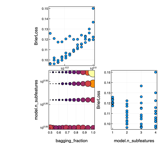
Predicting on new data using the optimized model:
predict(mach, Xnew)3-element UnivariateFiniteVector{Multiclass{3}, String, UInt32, Float64}:
UnivariateFinite{Multiclass{3}}(setosa=>1.0, versicolor=>0.0, virginica=>0.0)
UnivariateFinite{Multiclass{3}}(setosa=>0.85, versicolor=>0.137, virginica=>0.0133)
UnivariateFinite{Multiclass{3}}(setosa=>1.0, versicolor=>0.0, virginica=>0.0)Constructing linear pipelines
Reference: Composing Models
Constructing a linear (unbranching) pipeline with a learned target transformation/inverse transformation:
X, y = @load_reduced_ames
KNN = @load KNNRegressor
knn_with_target = TransformedTargetModel(model=KNN(K=3), transformer=Standardizer())
pipe = (X -> coerce(X, :age=>Continuous)) |> OneHotEncoder() |> knn_with_target
DeterministicPipeline(
f = Main.var"#15#16"(),
one_hot_encoder = OneHotEncoder(
features = Symbol[],
drop_last = false,
ordered_factor = true,
ignore = false),
transformed_target_model_deterministic = TransformedTargetModelDeterministic(
model = KNNRegressor(K = 3, …),
transformer = Standardizer(features = Symbol[], …),
inverse = nothing,
cache = true),
cache = true)Evaluating the pipeline (just as you would any other model):
pipe.one_hot_encoder.drop_last = true # mutate a nested hyper-parameter
evaluate(pipe, X, y, resampling=Holdout(), measure=RootMeanSquaredError(), verbosity=2)
PerformanceEvaluation object with these fields:
model, measure, operation, measurement, per_fold,
per_observation, fitted_params_per_fold,
report_per_fold, train_test_rows, resampling, repeats
Extract:
┌────────────────────────┬───────────┬─────────────┬───────────┐
│ measure │ operation │ measurement │ per_fold │
├────────────────────────┼───────────┼─────────────┼───────────┤
│ RootMeanSquaredError() │ predict │ 51200.0 │ [51200.0] │
└────────────────────────┴───────────┴─────────────┴───────────┘
Inspecting the learned parameters in a pipeline:
mach = machine(pipe, X, y) |> fit!
F = fitted_params(mach)
F.transformed_target_model_deterministic.model
(tree = NearestNeighbors.KDTree{StaticArraysCore.SVector{56, Float64}, Distances.Euclidean, Float64, StaticArraysCore.SVector{56, Float64}}
Number of points: 1456
Dimensions: 56
Metric: Distances.Euclidean(0.0)
Reordered: true,)Constructing a linear (unbranching) pipeline with a static (unlearned) target transformation/inverse transformation:
Tree = @load DecisionTreeRegressor pkg=DecisionTree verbosity=0
tree_with_target = TransformedTargetModel(model=Tree(),
                                          transformer=y -> log.(y),
                                          inverse = z -> exp.(z))
pipe2 = (X -> coerce(X, :age=>Continuous)) |> OneHotEncoder() |> tree_with_target;
Creating a homogeneous ensemble of models
Reference: Homogeneous Ensembles
X, y = @load_iris
Tree = @load DecisionTreeClassifier pkg=DecisionTree
tree = Tree()
forest = EnsembleModel(model=tree, bagging_fraction=0.8, n=300)
mach = machine(forest, X, y)
evaluate!(mach, measure=LogLoss())
PerformanceEvaluation object with these fields:
model, measure, operation, measurement, per_fold,
per_observation, fitted_params_per_fold,
report_per_fold, train_test_rows, resampling, repeats
Extract:
┌──────────────────────┬───────────┬─────────────┬─────────┬────────────────────
│ measure │ operation │ measurement │ 1.96*SE │ per_fold ⋯
├──────────────────────┼───────────┼─────────────┼─────────┼────────────────────
│ LogLoss( │ predict │ 0.421 │ 0.508 │ [3.89e-15, 3.89e- ⋯
│ tol = 2.22045e-16) │ │ │ │ ⋯
└──────────────────────┴───────────┴─────────────┴─────────┴────────────────────
1 column omitted
Performance curves
Generate a plot of performance, as a function of some hyperparameter (building on the preceding example)
Single performance curve:
r = range(forest, :n, lower=1, upper=1000, scale=:log10)
curve = learning_curve(mach,
                       range=r,
                       resampling=Holdout(),
                       resolution=50,
                       measure=LogLoss(),
                       verbosity=0)
(parameter_name = "n",
parameter_scale = :log10,
parameter_values = [1, 2, 3, 4, 5, 6, 7, 8, 10, 11 … 281, 324, 373, 429, 494, 569, 655, 754, 869, 1000],
measurements = [15.218431430960575, 6.608003121338145, 6.586508049790735, 6.557716641074733, 6.564643919186257, 6.554665209414641, 2.761309309001218, 1.998324925450971, 1.1640157211960025, 1.1635074923549868 … 1.2421921856299438, 1.2328289465607303, 1.232660936494746, 1.2387429252643096, 1.2351081888595659, 1.2366288097323843, 1.239044879729414, 1.2448612762613058, 1.2431957394563597, 1.2466258022771786],)using Plots
plot(curve.parameter_values, curve.measurements, xlab=curve.parameter_name, xscale=curve.parameter_scale)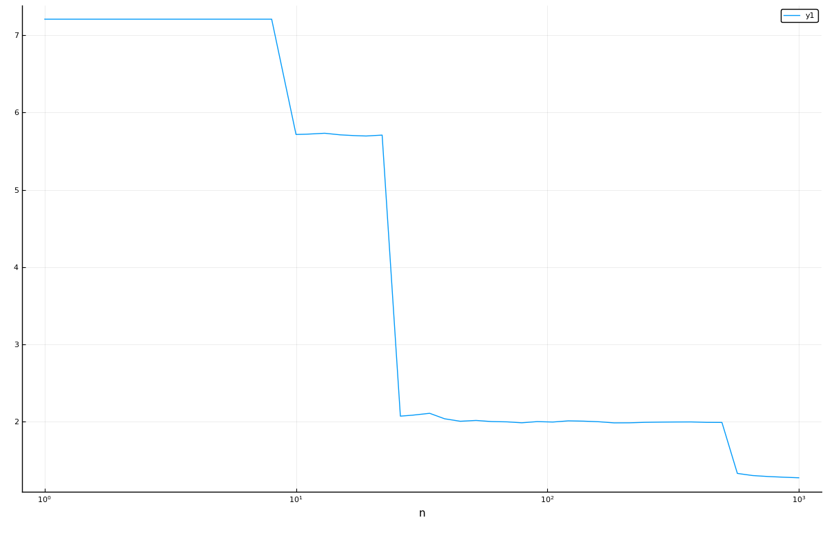
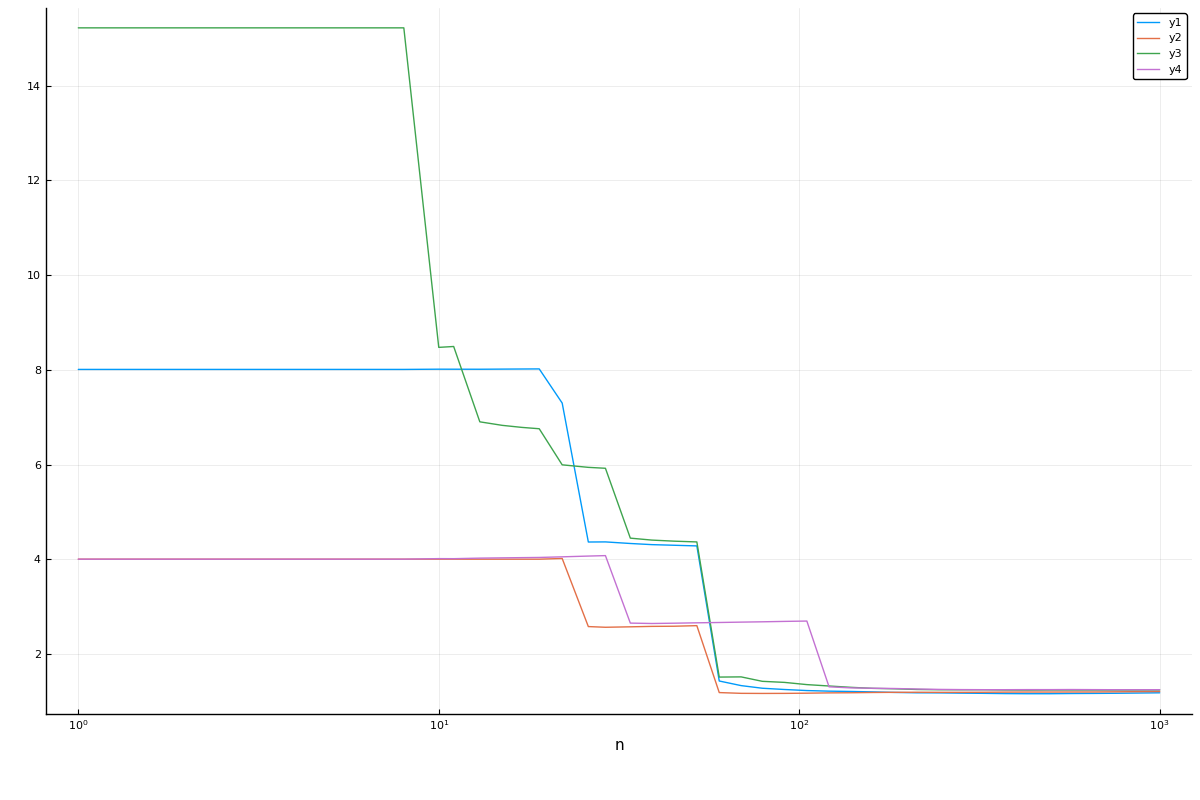
Multiple curves:
curve = learning_curve(mach,
                       range=r,
                       resampling=Holdout(),
                       measure=LogLoss(),
                       resolution=50,
                       rng_name=:rng,
                       rngs=4,
                       verbosity=0)
(parameter_name = "n",
parameter_scale = :log10,
parameter_values = [1, 2, 3, 4, 5, 6, 7, 8, 10, 11 … 281, 324, 373, 429, 494, 569, 655, 754, 869, 1000],
measurements = [4.004850376568572 8.009700753137146 16.820371581588002 8.009700753137146; 4.004850376568572 8.040507294495367 9.087929700674836 8.009700753137146; … ; 1.2032095186799414 1.231410971269136 1.2618260081921822 1.2771759492571848; 1.208361023670845 1.2299991814751527 1.264384762090153 1.278189281728243],)plot(curve.parameter_values, curve.measurements,
xlab=curve.parameter_name, xscale=curve.parameter_scale)