Common MLJ Workflows

Data ingestion

import RDatasets
channing = RDatasets.dataset("boot", "channing")
first(channing, 4)

4 rows × 5 columns

	Sex	Entry	Exit	Time	Cens
	Cat…	Int32	Int32	Int32	Int32
1	Male	782	909	127	1
2	Male	1020	1128	108	1
3	Male	856	969	113	1
4	Male	915	957	42	1

Inspecting metadata, including column scientific types:

schema(channing)

┌─────────┬────────────────────────────────┬───────────────┐
│ _.names │ _.types                        │ _.scitypes    │
├─────────┼────────────────────────────────┼───────────────┤
│ Sex     │ CategoricalValue{String,UInt8} │ Multiclass{2} │
│ Entry   │ Int32                          │ Count         │
│ Exit    │ Int32                          │ Count         │
│ Time    │ Int32                          │ Count         │
│ Cens    │ Int32                          │ Count         │
└─────────┴────────────────────────────────┴───────────────┘
_.nrows = 462

Unpacking data and correcting for wrong scitypes:

y, X =  unpack(channing,
               ==(:Exit),            # y is the :Exit column
               !=(:Time);            # X is the rest, except :Time
               :Exit=>Continuous,
               :Entry=>Continuous,
               :Cens=>Multiclass)
first(X, 4)

4 rows × 3 columns

	Sex	Entry	Cens
	Cat…	Float64	Cat…
1	Male	782.0	1
2	Male	1020.0	1
3	Male	856.0	1
4	Male	915.0	1

Note: Before julia 1.2, replace !=(:Time) with col -> col != :Time.

y[1:4]

4-element Array{Float64,1}:
  909.0
 1128.0
  969.0
  957.0

Loading a built-in supervised dataset:

X, y = @load_iris;
selectrows(X, 1:4) # selectrows works for any Tables.jl table

(sepal_length = [5.1, 4.9, 4.7, 4.6],
 sepal_width = [3.5, 3.0, 3.2, 3.1],
 petal_length = [1.4, 1.4, 1.3, 1.5],
 petal_width = [0.2, 0.2, 0.2, 0.2],)

y[1:4]

4-element CategoricalArray{String,1,UInt32}:
 "setosa"
 "setosa"
 "setosa"
 "setosa"

Model search

Reference: Model Search

Searching for a supervised model:

X, y = @load_boston
models(matching(X, y))

54-element Array{NamedTuple{(:name, :package_name, :is_supervised, :docstring, :hyperparameter_ranges, :hyperparameter_types, :hyperparameters, :implemented_methods, :is_pure_julia, :is_wrapper, :load_path, :package_license, :package_url, :package_uuid, :prediction_type, :supports_online, :supports_weights, :input_scitype, :target_scitype, :output_scitype),T} where T<:Tuple,1}:
 (name = ARDRegressor, package_name = ScikitLearn, ... )                
 (name = AdaBoostRegressor, package_name = ScikitLearn, ... )           
 (name = BaggingRegressor, package_name = ScikitLearn, ... )            
 (name = BayesianRidgeRegressor, package_name = ScikitLearn, ... )      
 (name = ConstantRegressor, package_name = MLJModels, ... )             
 (name = DecisionTreeRegressor, package_name = DecisionTree, ... )      
 (name = DeterministicConstantRegressor, package_name = MLJModels, ... )
 (name = DummyRegressor, package_name = ScikitLearn, ... )              
 (name = ElasticNetCVRegressor, package_name = ScikitLearn, ... )       
 (name = ElasticNetRegressor, package_name = MLJLinearModels, ... )     
 ⋮                                                                      
 (name = RidgeRegressor, package_name = MultivariateStats, ... )        
 (name = RidgeRegressor, package_name = ScikitLearn, ... )              
 (name = RobustRegressor, package_name = MLJLinearModels, ... )         
 (name = SGDRegressor, package_name = ScikitLearn, ... )                
 (name = SVMLinearRegressor, package_name = ScikitLearn, ... )          
 (name = SVMNuRegressor, package_name = ScikitLearn, ... )              
 (name = SVMRegressor, package_name = ScikitLearn, ... )                
 (name = TheilSenRegressor, package_name = ScikitLearn, ... )           
 (name = XGBoostRegressor, package_name = XGBoost, ... )

models(matching(X, y))[6]

CART decision tree regressor.
→ based on [DecisionTree](https://github.com/bensadeghi/DecisionTree.jl).
→ do `@load DecisionTreeRegressor pkg="DecisionTree"` to use the model.
→ do `?DecisionTreeRegressor` for documentation.
(name = "DecisionTreeRegressor",
 package_name = "DecisionTree",
 is_supervised = true,
 docstring = "CART decision tree regressor.\n→ based on [DecisionTree](https://github.com/bensadeghi/DecisionTree.jl).\n→ do `@load DecisionTreeRegressor pkg=\"DecisionTree\"` to use the model.\n→ do `?DecisionTreeRegressor` for documentation.",
 hyperparameter_ranges = (nothing, nothing, nothing, nothing, nothing, nothing, nothing),
 hyperparameter_types = ("Int64", "Int64", "Int64", "Float64", "Int64", "Bool", "Float64"),
 hyperparameters = (:max_depth, :min_samples_leaf, :min_samples_split, :min_purity_increase, :n_subfeatures, :post_prune, :merge_purity_threshold),
 implemented_methods = Symbol[:clean!, :fit, :fitted_params, :predict],
 is_pure_julia = true,
 is_wrapper = false,
 load_path = "MLJModels.DecisionTree_.DecisionTreeRegressor",
 package_license = "MIT",
 package_url = "https://github.com/bensadeghi/DecisionTree.jl",
 package_uuid = "7806a523-6efd-50cb-b5f6-3fa6f1930dbb",
 prediction_type = :deterministic,
 supports_online = false,
 supports_weights = false,
 input_scitype = Table{_s23} where _s23<:Union{AbstractArray{_s25,1} where _s25<:Continuous, AbstractArray{_s25,1} where _s25<:Count, AbstractArray{_s25,1} where _s25<:OrderedFactor},
 target_scitype = AbstractArray{Continuous,1},
 output_scitype = Unknown,)

Instantiating a model

Reference: Getting Started

@load DecisionTreeClassifier
model = DecisionTreeClassifier(min_samples_split=5, max_depth=4)

DecisionTreeClassifier(
    max_depth = 4,
    min_samples_leaf = 1,
    min_samples_split = 5,
    min_purity_increase = 0.0,
    n_subfeatures = 0,
    post_prune = false,
    merge_purity_threshold = 1.0,
    pdf_smoothing = 0.0,
    display_depth = 5) @412

model = @load DecisionTreeClassifier
model.min_samples_split = 5
model.max_depth = 4

Evaluating a model

Reference: Evaluating Model Performance

X, y = @load_boston
model = @load KNNRegressor
evaluate(model, X, y, resampling=CV(nfolds=5), measure=[rms, mav])

┌───────────┬───────────────┬───────────────────────────────┐
│ _.measure │ _.measurement │ _.per_fold                    │
├───────────┼───────────────┼───────────────────────────────┤
│ rms       │ 8.77          │ [8.53, 8.8, 10.7, 9.43, 5.59] │
│ mae       │ 6.02          │ [6.52, 5.7, 7.65, 6.09, 4.11] │
└───────────┴───────────────┴───────────────────────────────┘
_.per_observation = [missing, missing]

Basic fit/evaluate/predict by hand:

Reference: Getting Started, Machines, Evaluating Model Performance, Performance Measures

import RDatasets
vaso = RDatasets.dataset("robustbase", "vaso"); # a DataFrame
first(vaso, 3)

3 rows × 3 columns

	Volume	Rate	Y
	Float64	Float64	Int64
1	3.7	0.825	1
2	3.5	1.09	1
3	1.25	2.5	1

y, X = unpack(vaso, ==(:Y), c -> true; :Y => Multiclass)

tree_model = @load DecisionTreeClassifier

Bind the model and data together in a machine , which will additionally store the learned parameters (fitresults) when fit:

tree = machine(tree_model, X, y)

Machine{DecisionTreeClassifier} @441 trained 0 times.
  args: 
    1:	Source @543 ⏎ `Table{AbstractArray{Continuous,1}}`
    2:	Source @516 ⏎ `AbstractArray{Multiclass{2},1}`

Split row indices into training and evaluation rows:

train, test = partition(eachindex(y), 0.7, shuffle=true, rng=1234); # 70:30 split

([27, 28, 30, 31, 32, 18, 21, 9, 26, 14  …  7, 39, 2, 37, 1, 8, 19, 25, 35, 34], [22, 13, 11, 4, 10, 16, 3, 20, 29, 23, 12, 24])

Fit on train and evaluate on test:

fit!(tree, rows=train)
yhat = predict(tree, X[test,:])
mean(cross_entropy(yhat, y[test]))

6.5216583816514975

Predict on new data:

Xnew = (Volume=3*rand(3), Rate=3*rand(3))
predict(tree, Xnew)      # a vector of distributions

3-element MLJBase.UnivariateFiniteArray{Multiclass{2},Int64,UInt32,Float64,1}:
 UnivariateFinite{Multiclass{2}}(0=>0.9, 1=>0.1)
 UnivariateFinite{Multiclass{2}}(0=>0.0, 1=>1.0)
 UnivariateFinite{Multiclass{2}}(0=>0.9, 1=>0.1)

predict_mode(tree, Xnew) # a vector of point-predictions

3-element CategoricalArray{Int64,1,UInt32}:
 0
 1
 0

More performance evaluation examples

import LossFunctions.ZeroOneLoss

Evaluating model + data directly:

evaluate(tree_model, X, y,
         resampling=Holdout(fraction_train=0.7, shuffle=true, rng=1234),
         measure=[cross_entropy, ZeroOneLoss()])

┌───────────────┬───────────────┬────────────┐
│ _.measure     │ _.measurement │ _.per_fold │
├───────────────┼───────────────┼────────────┤
│ cross_entropy │ 6.52          │ [6.52]     │
│ ZeroOneLoss   │ 0.417         │ [0.417]    │
└───────────────┴───────────────┴────────────┘
_.per_observation = [[[0.105, 36.0, ..., 1.3]], [[0.0, 1.0, ..., 1.0]]]

If a machine is already defined, as above:

evaluate!(tree,
          resampling=Holdout(fraction_train=0.7, shuffle=true, rng=1234),
          measure=[cross_entropy, ZeroOneLoss()])

┌───────────────┬───────────────┬────────────┐
│ _.measure     │ _.measurement │ _.per_fold │
├───────────────┼───────────────┼────────────┤
│ cross_entropy │ 6.52          │ [6.52]     │
│ ZeroOneLoss   │ 0.417         │ [0.417]    │
└───────────────┴───────────────┴────────────┘
_.per_observation = [[[0.105, 36.0, ..., 1.3]], [[0.0, 1.0, ..., 1.0]]]

Using cross-validation:

evaluate!(tree, resampling=CV(nfolds=5, shuffle=true, rng=1234),
          measure=[cross_entropy, ZeroOneLoss()])

┌───────────────┬───────────────┬───────────────────────────────────┐
│ _.measure     │ _.measurement │ _.per_fold                        │
├───────────────┼───────────────┼───────────────────────────────────┤
│ cross_entropy │ 2.47          │ [9.25, 0.598, 0.912, 1.07, 0.546] │
│ ZeroOneLoss   │ 0.432         │ [0.5, 0.375, 0.5, 0.5, 0.286]     │
└───────────────┴───────────────┴───────────────────────────────────┘
_.per_observation = [[[2.22e-16, 0.944, ..., 2.22e-16], [0.847, 0.56, ..., 0.56], [0.194, 2.22e-16, ..., 0.223], [2.01, 2.01, ..., 0.143], [0.405, 0.405, ..., 1.1]], [[0.0, 1.0, ..., 0.0], [1.0, 0.0, ..., 0.0], [0.0, 0.0, ..., 0.0], [1.0, 1.0, ..., 0.0], [0.0, 0.0, ..., 1.0]]]

With user-specified train/test pairs of row indices:

f1, f2, f3 = 1:13, 14:26, 27:36
pairs = [(f1, vcat(f2, f3)), (f2, vcat(f3, f1)), (f3, vcat(f1, f2))];
evaluate!(tree,
          resampling=pairs,
          measure=[cross_entropy, ZeroOneLoss()])

┌───────────────┬───────────────┬───────────────────────┐
│ _.measure     │ _.measurement │ _.per_fold            │
├───────────────┼───────────────┼───────────────────────┤
│ cross_entropy │ 5.88          │ [2.16, 11.0, 4.51]    │
│ ZeroOneLoss   │ 0.241         │ [0.304, 0.304, 0.115] │
└───────────────┴───────────────┴───────────────────────┘
_.per_observation = [[[0.154, 0.154, ..., 0.154], [2.22e-16, 36.0, ..., 2.22e-16], [2.22e-16, 2.22e-16, ..., 0.693]], [[0.0, 0.0, ..., 0.0], [0.0, 1.0, ..., 0.0], [0.0, 0.0, ..., 0.0]]]

Changing a hyperparameter and re-evaluating:

tree_model.max_depth = 3
evaluate!(tree,
          resampling=CV(nfolds=5, shuffle=true, rng=1234),
          measure=[cross_entropy, ZeroOneLoss()])

┌───────────────┬───────────────┬────────────────────────────────────┐
│ _.measure     │ _.measurement │ _.per_fold                         │
├───────────────┼───────────────┼────────────────────────────────────┤
│ cross_entropy │ 2.23          │ [9.18, 0.484, 0.427, 0.564, 0.488] │
│ ZeroOneLoss   │ 0.307         │ [0.375, 0.25, 0.25, 0.375, 0.286]  │
└───────────────┴───────────────┴────────────────────────────────────┘
_.per_observation = [[[2.22e-16, 1.32, ..., 2.22e-16], [2.22e-16, 0.318, ..., 0.318], [0.405, 2.22e-16, ..., 2.22e-16], [1.5, 1.5, ..., 2.22e-16], [0.636, 2.22e-16, ..., 0.754]], [[0.0, 1.0, ..., 0.0], [0.0, 0.0, ..., 0.0], [0.0, 0.0, ..., 0.0], [1.0, 1.0, ..., 0.0], [0.0, 0.0, ..., 1.0]]]

Inspecting training results

Fit a ordinary least square model to some synthetic data:

x1 = rand(100)
x2 = rand(100)

X = (x1=x1, x2=x2)
y = x1 - 2x2 + 0.1*rand(100);

ols_model = @load LinearRegressor pkg=GLM
ols =  machine(ols_model, X, y)
fit!(ols)

Machine{LinearRegressor} @223 trained 1 time.
  args: 
    1:	Source @582 ⏎ `Table{AbstractArray{Continuous,1}}`
    2:	Source @879 ⏎ `AbstractArray{Continuous,1}`

Get a named tuple representing the learned parameters, human-readable if appropriate:

fitted_params(ols)

(coef = [1.0080655105944518, -2.025251774924713],
 intercept = 0.06000539881652656,)

Get other training-related information:

report(ols)

(deviance = 0.08410497179295867,
 dof_residual = 97.0,
 stderror = [0.011286607269176215, 0.009862863065673438, 0.007325240278907562],
 vcov = [0.0001273875036486214 -1.1714998269445943e-5 -5.0936212789785576e-5; -1.1714998269445943e-5 9.727606785222524e-5 -4.398360474974536e-5; -5.0936212789785576e-5 -4.398360474974536e-5 5.365914514372973e-5],)

Basic fit/transform for unsupervised models

Load data:

X, y = @load_iris
train, test = partition(eachindex(y), 0.97, shuffle=true, rng=123)

([125, 100, 130, 9, 70, 148, 39, 64, 6, 107  …  110, 59, 139, 21, 112, 144, 140, 72, 109, 41], [106, 147, 47, 5])

Instantiate and fit the model/machine:

@load PCA
pca_model = PCA(maxoutdim=2)
pca = machine(pca_model, X)
fit!(pca, rows=train)

Machine{PCA} @626 trained 1 time.
  args: 
    1:	Source @078 ⏎ `Table{AbstractArray{Continuous,1}}`

Transform selected data bound to the machine:

transform(pca, rows=test);

(x1 = [-3.3942826854483243, -1.5219827578765068, 2.538247455185219, 2.7299639893931373],
 x2 = [0.5472450223745241, -0.36842368617126214, 0.5199299511335698, 0.3448466122232363],)

Transform new data:

Xnew = (sepal_length=rand(3), sepal_width=rand(3),
        petal_length=rand(3), petal_width=rand(3));
transform(pca, Xnew)

(x1 = [5.056670239157379, 4.880272282118678, 5.156522261208207],
 x2 = [-5.057408724542798, -4.948610876550504, -4.95956799333649],)

Inverting learned transformations

y = rand(100);
stand_model = UnivariateStandardizer()
stand = machine(stand_model, y)
fit!(stand)
z = transform(stand, y);
@assert inverse_transform(stand, z) ≈ y # true

[ Info: Training Machine{UnivariateStandardizer} @541.

Nested hyperparameter tuning

Reference: Tuning Models

Define a model with nested hyperparameters:

tree_model = @load DecisionTreeClassifier
forest_model = EnsembleModel(atom=tree_model, n=300)

ProbabilisticEnsembleModel(
    atom = DecisionTreeClassifier(
            max_depth = -1,
            min_samples_leaf = 1,
            min_samples_split = 2,
            min_purity_increase = 0.0,
            n_subfeatures = 0,
            post_prune = false,
            merge_purity_threshold = 1.0,
            pdf_smoothing = 0.0,
            display_depth = 5),
    atomic_weights = Float64[],
    bagging_fraction = 0.8,
    rng = MersenneTwister(UInt32[0xf88b2cd5, 0x0b67973f, 0xa0e4f6c0, 0x05d66c97]) @ 25,
    n = 300,
    acceleration = CPU1{Nothing}(nothing),
    out_of_bag_measure = Any[]) @154

Inspect all hyperparameters, even nested ones (returns nested named tuple):

params(forest_model)

(atom = (max_depth = -1,
         min_samples_leaf = 1,
         min_samples_split = 2,
         min_purity_increase = 0.0,
         n_subfeatures = 0,
         post_prune = false,
         merge_purity_threshold = 1.0,
         pdf_smoothing = 0.0,
         display_depth = 5,),
 atomic_weights = Float64[],
 bagging_fraction = 0.8,
 rng = MersenneTwister(UInt32[0xf88b2cd5, 0x0b67973f, 0xa0e4f6c0, 0x05d66c97]) @ 25,
 n = 300,
 acceleration = CPU1{Nothing}(nothing),
 out_of_bag_measure = Any[],)

Define ranges for hyperparameters to be tuned:

r1 = range(forest_model, :bagging_fraction, lower=0.5, upper=1.0, scale=:log10)

MLJBase.NumericRange(Float64, :bagging_fraction, ... )

r2 = range(forest_model, :(atom.n_subfeatures), lower=1, upper=4) # nested

MLJBase.NumericRange(Int64, :(atom.n_subfeatures), ... )

Wrap the model in a tuning strategy:

tuned_forest = TunedModel(model=forest_model,
                          tuning=Grid(resolution=12),
                          resampling=CV(nfolds=6),
                          ranges=[r1, r2],
                          measure=cross_entropy)

ProbabilisticTunedModel(
    model = ProbabilisticEnsembleModel(
            atom = DecisionTreeClassifier @308,
            atomic_weights = Float64[],
            bagging_fraction = 0.8,
            rng = MersenneTwister(UInt32[0xf88b2cd5, 0x0b67973f, 0xa0e4f6c0, 0x05d66c97]) @ 25,
            n = 300,
            acceleration = CPU1{Nothing}(nothing),
            out_of_bag_measure = Any[]),
    tuning = Grid(
            goal = nothing,
            resolution = 12,
            shuffle = true,
            rng = MersenneTwister(UInt32[0xf88b2cd5, 0x0b67973f, 0xa0e4f6c0, 0x05d66c97]) @ 25),
    resampling = CV(
            nfolds = 6,
            shuffle = false,
            rng = MersenneTwister(UInt32[0xf88b2cd5, 0x0b67973f, 0xa0e4f6c0, 0x05d66c97]) @ 25),
    measure = cross_entropy(
            eps = 2.220446049250313e-16),
    weights = nothing,
    operation = MLJModelInterface.predict,
    range = MLJBase.NumericRange{T,MLJBase.Bounded,Symbol} where T[NumericRange{Float64,…} @743, NumericRange{Int64,…} @529],
    train_best = true,
    repeats = 1,
    n = nothing,
    acceleration = CPU1{Nothing}(nothing),
    acceleration_resampling = CPU1{Nothing}(nothing),
    check_measure = true) @957

Bound the wrapped model to data:

tuned = machine(tuned_forest, X, y)

Machine{ProbabilisticTunedModel{Grid,…}} @057 trained 0 times.
  args: 
    1:	Source @399 ⏎ `Table{AbstractArray{Continuous,1}}`
    2:	Source @610 ⏎ `AbstractArray{Multiclass{3},1}`

Fitting the resultant machine optimizes the hyperparameters specified in range, using the specified tuning and resampling strategies and performance measure (possibly a vector of measures), and retrains on all data bound to the machine:

fit!(tuned)

Machine{ProbabilisticTunedModel{Grid,…}} @057 trained 1 time.
  args: 
    1:	Source @399 ⏎ `Table{AbstractArray{Continuous,1}}`
    2:	Source @610 ⏎ `AbstractArray{Multiclass{3},1}`

Inspecting the optimal model:

F = fitted_params(tuned)

(best_model = ProbabilisticEnsembleModel{DecisionTreeClassifier} @788,
 best_fitted_params = (fitresult = WrappedEnsemble{Tuple{Node{Float64,…},…},…} @403,),)

F.best_model

ProbabilisticEnsembleModel(
    atom = DecisionTreeClassifier(
            max_depth = -1,
            min_samples_leaf = 1,
            min_samples_split = 2,
            min_purity_increase = 0.0,
            n_subfeatures = 3,
            post_prune = false,
            merge_purity_threshold = 1.0,
            pdf_smoothing = 0.0,
            display_depth = 5),
    atomic_weights = Float64[],
    bagging_fraction = 0.5,
    rng = MersenneTwister(UInt32[0xf88b2cd5, 0x0b67973f, 0xa0e4f6c0, 0x05d66c97]) @ 116,
    n = 300,
    acceleration = CPU1{Nothing}(nothing),
    out_of_bag_measure = Any[]) @788

Inspecting details of tuning procedure:

report(tuned)

(best_model = ProbabilisticEnsembleModel{DecisionTreeClassifier} @788,
 best_result = (measure = MLJBase.CrossEntropy{Float64}[cross_entropy],
                measurement = [0.15397085904257765],),
 best_report = (measures = Any[],
                oob_measurements = missing,),
 history = Tuple{MLJ.ProbabilisticEnsembleModel{MLJModels.DecisionTree_.DecisionTreeClassifier},NamedTuple{(:measure, :measurement),Tuple{Array{MLJBase.CrossEntropy{Float64},1},Array{Float64,1}}}}[(ProbabilisticEnsembleModel{DecisionTreeClassifier} @772, (measure = [cross_entropy], measurement = [0.17603247979396464])), (ProbabilisticEnsembleModel{DecisionTreeClassifier} @976, (measure = [cross_entropy], measurement = [0.20597799028392946])), (ProbabilisticEnsembleModel{DecisionTreeClassifier} @175, (measure = [cross_entropy], measurement = [0.205612763112393])), (ProbabilisticEnsembleModel{DecisionTreeClassifier} @182, (measure = [cross_entropy], measurement = [0.4363170110551698])), (ProbabilisticEnsembleModel{DecisionTreeClassifier} @603, (measure = [cross_entropy], measurement = [0.20522158315704375])), (ProbabilisticEnsembleModel{DecisionTreeClassifier} @160, (measure = [cross_entropy], measurement = [0.1643147076037652])), (ProbabilisticEnsembleModel{DecisionTreeClassifier} @967, (measure = [cross_entropy], measurement = [0.6669237418022097])), (ProbabilisticEnsembleModel{DecisionTreeClassifier} @843, (measure = [cross_entropy], measurement = [0.4261498013589768])), (ProbabilisticEnsembleModel{DecisionTreeClassifier} @073, (measure = [cross_entropy], measurement = [0.428113404630653])), (ProbabilisticEnsembleModel{DecisionTreeClassifier} @322, (measure = [cross_entropy], measurement = [0.4317342281689274]))  …  (ProbabilisticEnsembleModel{DecisionTreeClassifier} @758, (measure = [cross_entropy], measurement = [0.16714541521874068])), (ProbabilisticEnsembleModel{DecisionTreeClassifier} @346, (measure = [cross_entropy], measurement = [0.18059837332843945])), (ProbabilisticEnsembleModel{DecisionTreeClassifier} @823, (measure = [cross_entropy], measurement = [0.4106428771878206])), (ProbabilisticEnsembleModel{DecisionTreeClassifier} @831, (measure = [cross_entropy], measurement = [0.21609321692467695])), (ProbabilisticEnsembleModel{DecisionTreeClassifier} @185, (measure = [cross_entropy], measurement = [0.20591254443180382])), (ProbabilisticEnsembleModel{DecisionTreeClassifier} @016, (measure = [cross_entropy], measurement = [0.8862361486830467])), (ProbabilisticEnsembleModel{DecisionTreeClassifier} @131, (measure = [cross_entropy], measurement = [0.21259522223663327])), (ProbabilisticEnsembleModel{DecisionTreeClassifier} @242, (measure = [cross_entropy], measurement = [0.41331119467751326])), (ProbabilisticEnsembleModel{DecisionTreeClassifier} @676, (measure = [cross_entropy], measurement = [0.18818233525930075])), (ProbabilisticEnsembleModel{DecisionTreeClassifier} @281, (measure = [cross_entropy], measurement = [0.21418075167561004]))],
 plotting = (parameter_names = ["bagging_fraction", "atom.n_subfeatures"],
             parameter_scales = Symbol[:log10, :linear],
             parameter_values = Any[0.6040447222022236 2; 0.6040447222022236 1; … ; 0.7297400528407231 2; 0.9389309106617063 1],
             measurements = [0.17603247979396464, 0.20597799028392946, 0.205612763112393, 0.4363170110551698, 0.20522158315704375, 0.1643147076037652, 0.6669237418022097, 0.4261498013589768, 0.428113404630653, 0.4317342281689274  …  0.16714541521874068, 0.18059837332843945, 0.4106428771878206, 0.21609321692467695, 0.20591254443180382, 0.8862361486830467, 0.21259522223663327, 0.41331119467751326, 0.18818233525930075, 0.21418075167561004],),)

Visualizing these results:

using Plots
plot(tuned)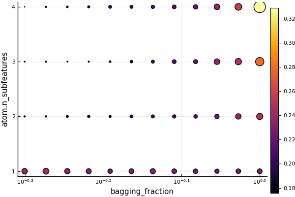

Predicting on new data using the optimized model:

predict(tuned, Xnew)

3-element Array{UnivariateFinite{Multiclass{3},String,UInt32,Float64},1}:
 UnivariateFinite{Multiclass{3}}(versicolor=>0.0, virginica=>0.0, setosa=>1.0)
 UnivariateFinite{Multiclass{3}}(versicolor=>0.0, virginica=>0.0, setosa=>1.0)
 UnivariateFinite{Multiclass{3}}(versicolor=>0.0, virginica=>0.0, setosa=>1.0)

Constructing a linear pipeline

Reference: Composing Models

Constructing a linear (unbranching) pipeline with a learned target transformation/inverse transformation:

X, y = @load_reduced_ames
@load KNNRegressor
pipe = @pipeline(X -> coerce(X, :age=>Continuous),
                 OneHotEncoder,
                 KNNRegressor(K=3),
                 target = UnivariateStandardizer)

Pipeline378(
    one_hot_encoder = OneHotEncoder(
            features = Symbol[],
            drop_last = false,
            ordered_factor = true,
            ignore = false),
    knn_regressor = KNNRegressor(
            K = 3,
            algorithm = :kdtree,
            metric = Distances.Euclidean(0.0),
            leafsize = 10,
            reorder = true,
            weights = :uniform),
    target = UnivariateStandardizer()) @643

Evaluating the pipeline (just as you would any other model):

pipe.knn_regressor.K = 2
pipe.one_hot_encoder.drop_last = true
evaluate(pipe, X, y, resampling=Holdout(), measure=rms, verbosity=2)

┌───────────┬───────────────┬────────────┐
│ _.measure │ _.measurement │ _.per_fold │
├───────────┼───────────────┼────────────┤
│ rms       │ 53100.0       │ [53100.0]  │
└───────────┴───────────────┴────────────┘
_.per_observation = [missing]

Inspecting the learned parameters in a pipeline:

mach = machine(pipe, X, y) |> fit!
F = fitted_params(mach)
F.one_hot_encoder

(fitresult = OneHotEncoderResult @660,)

Constructing a linear (unbranching) pipeline with a static (unlearned) target transformation/inverse transformation:

@load DecisionTreeRegressor
pipe2 = @pipeline(X -> coerce(X, :age=>Continuous),
                  OneHotEncoder,
                  DecisionTreeRegressor(max_depth=4),
                  target = y -> log.(y),
                  inverse = z -> exp.(z))

Pipeline389(
    one_hot_encoder = OneHotEncoder(
            features = Symbol[],
            drop_last = false,
            ordered_factor = true,
            ignore = false),
    decision_tree_regressor = DecisionTreeRegressor(
            max_depth = 4,
            min_samples_leaf = 5,
            min_samples_split = 2,
            min_purity_increase = 0.0,
            n_subfeatures = 0,
            post_prune = false,
            merge_purity_threshold = 1.0),
    target = WrappedFunction(
            f = getfield(Main.ex-workflows, Symbol("##28#29"))()),
    inverse = WrappedFunction(
            f = getfield(Main.ex-workflows, Symbol("##30#31"))())) @469

Creating a homogeneous ensemble of models

Reference: Homogeneous Ensembles

X, y = @load_iris
tree_model = @load DecisionTreeClassifier
forest_model = EnsembleModel(atom=tree_model, bagging_fraction=0.8, n=300)
forest = machine(forest_model, X, y)
evaluate!(forest, measure=cross_entropy)

┌───────────────┬───────────────┬────────────────────────────────────────────────┐
│ _.measure     │ _.measurement │ _.per_fold                                     │
├───────────────┼───────────────┼────────────────────────────────────────────────┤
│ cross_entropy │ 0.632         │ [3.66e-15, 3.66e-15, 0.302, 1.63, 1.56, 0.297] │
└───────────────┴───────────────┴────────────────────────────────────────────────┘
_.per_observation = [[[3.66e-15, 3.66e-15, ..., 3.66e-15], [3.66e-15, 3.66e-15, ..., 3.66e-15], [0.0339, 0.00669, ..., 3.66e-15], [3.66e-15, 0.151, ..., 3.66e-15], [3.66e-15, 0.0305, ..., 3.66e-15], [0.0101, 0.416, ..., 0.0236]]]

Performance curves

Generate a plot of performance, as a function of some hyperparameter (building on the preceding example)

Single performance curve:

r = range(forest_model, :n, lower=1, upper=1000, scale=:log10)
curve = learning_curve(forest,
                            range=r,
                            resampling=Holdout(),
                            resolution=50,
                            measure=cross_entropy,
                            verbosity=0)

(parameter_name = "n",
 parameter_scale = :log10,
 parameter_values = [1, 2, 3, 4, 5, 6, 7, 8, 10, 11  …  281, 324, 373, 429, 494, 569, 655, 754, 869, 1000],
 measurements = [9.611640903764574, 8.040507294495367, 8.02772142460862, 8.022486623023893, 8.019618244306665, 8.02772142460862, 8.024655074764755, 8.022486623023893, 6.553873181941727, 6.560335130753632  …  1.1822565516562635, 1.1852716578354472, 1.186755090025792, 1.1911180135449058, 1.1950386495322065, 1.1993836461745688, 1.2009277074726263, 1.202970009947571, 1.205323550069436, 1.207019155287965],)

using Plots
plot(curve.parameter_values, curve.measurements, xlab=curve.parameter_name, xscale=curve.parameter_scale)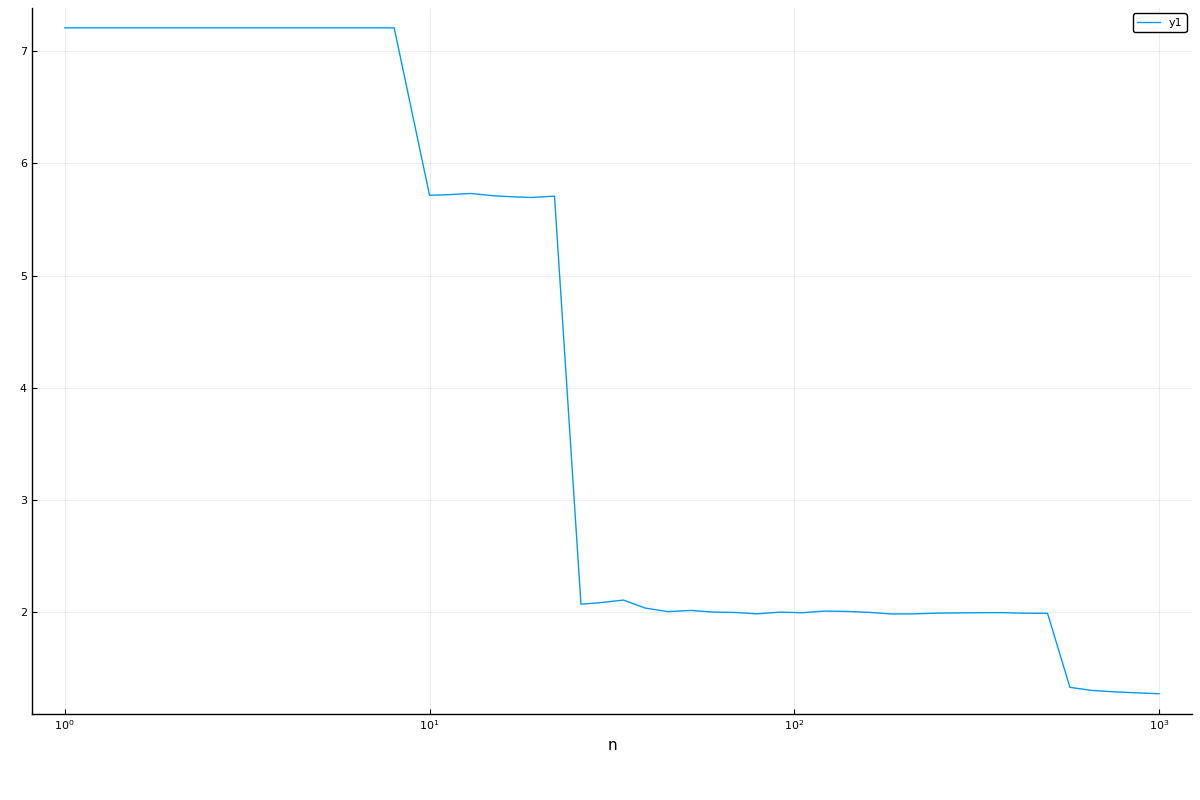

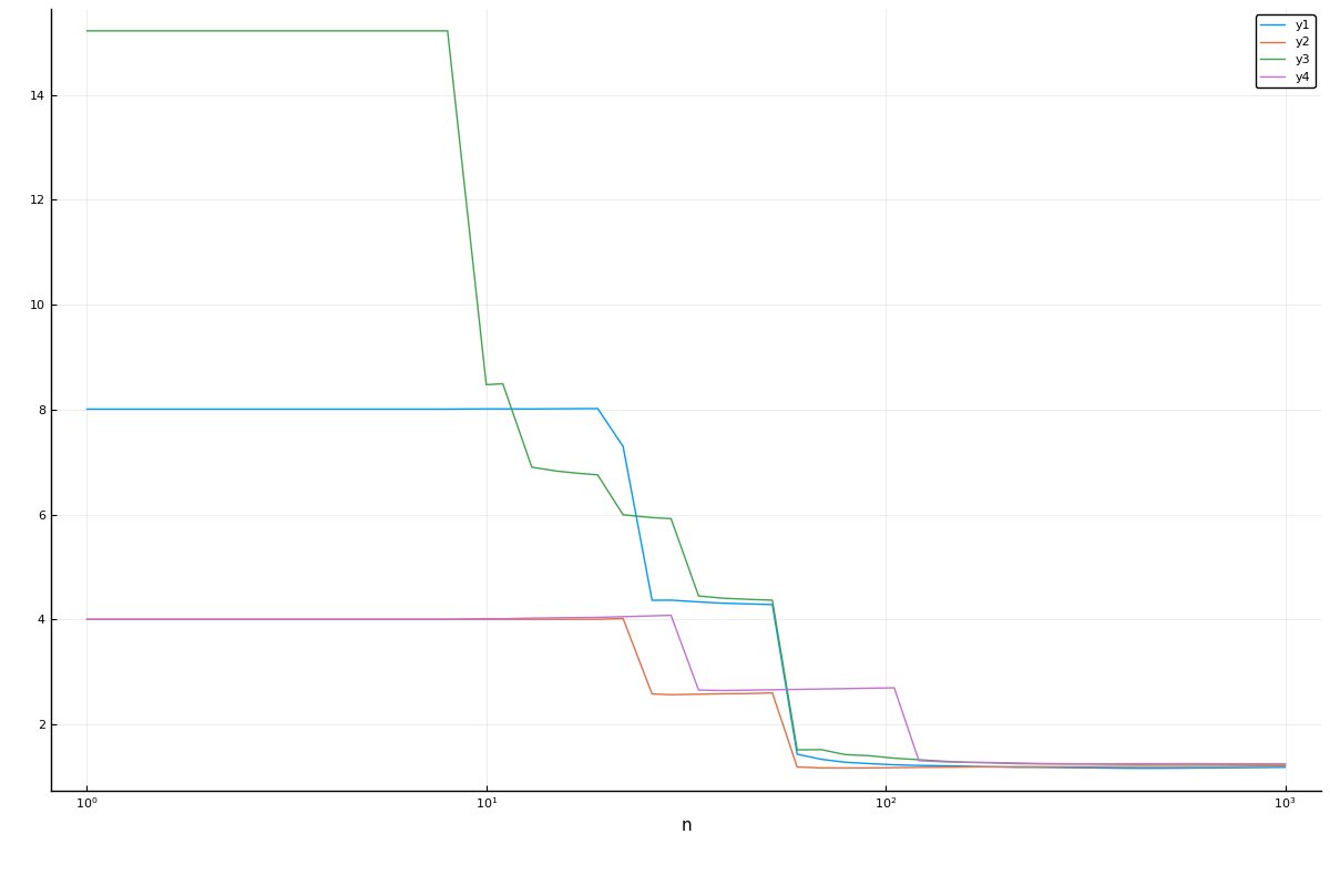
Multiple curves:

curve = learning_curve(forest,
                       range=r,
                       resampling=Holdout(),
                       measure=cross_entropy,
                       resolution=50,
                       rng_name=:rng,
                       rngs=4,
                       verbosity=0)

(parameter_name = "n",
 parameter_scale = :log10,
 parameter_values = [1, 2, 3, 4, 5, 6, 7, 8, 10, 11  …  281, 324, 373, 429, 494, 569, 655, 754, 869, 1000],
 measurements = [8.009700753137146 4.004850376568572 15.218431430960575 4.004850376568572; 8.009700753137146 4.004850376568572 15.218431430960575 4.004850376568572; … ; 1.181266790241928 1.2114602474428133 1.2536651226302669 1.2487615743781697; 1.1844915191838603 1.2144600734588165 1.2561310362994738 1.2504268375756997],)

plot(curve.parameter_values, curve.measurements,
xlab=curve.parameter_name, xscale=curve.parameter_scale)