Getting Started

For an outline of MLJ's goals and features, see the Introduction.

This section introduces the most basic MLJ operations and concepts. It assumes MJL has been successfully installed. See Installation if this is not the case.

Choosing and evaluating a model

To load some demonstration data, add RDatasets to your load path and enter

julia> import RDatasets

julia> iris = RDatasets.dataset("datasets", "iris"); # a DataFrame

and then split the data into input and target parts:

julia> using MLJ

julia> y, X = unpack(iris, ==(:Species), colname -> true);

julia> first(X, 3) |> pretty
┌─────────────┬────────────┬─────────────┬────────────┐
│ SepalLength │ SepalWidth │ PetalLength │ PetalWidth │
│ Float64     │ Float64    │ Float64     │ Float64    │
│ Continuous  │ Continuous │ Continuous  │ Continuous │
├─────────────┼────────────┼─────────────┼────────────┤
│ 5.1         │ 3.5        │ 1.4         │ 0.2        │
│ 4.9         │ 3.0        │ 1.4         │ 0.2        │
│ 4.7         │ 3.2        │ 1.3         │ 0.2        │
└─────────────┴────────────┴─────────────┴────────────┘

To list all models available in MLJ's model registry do models(). Listing the models compatible with the present data:

julia> models(matching(X,y))
42-element Array{NamedTuple{(:name, :package_name, :is_supervised, :docstring, :hyperparameter_ranges, :hyperparameter_types, :hyperparameters, :implemented_methods, :is_pure_julia, :is_wrapper, :load_path, :package_license, :package_url, :package_uuid, :prediction_type, :supports_online, :supports_weights, :input_scitype, :target_scitype, :output_scitype),T} where T<:Tuple,1}:
 (name = AdaBoostClassifier, package_name = ScikitLearn, ... )
 (name = AdaBoostStumpClassifier, package_name = DecisionTree, ... )
 (name = BaggingClassifier, package_name = ScikitLearn, ... )
 (name = BayesianLDA, package_name = MultivariateStats, ... )
 (name = BayesianLDA, package_name = ScikitLearn, ... )
 (name = BayesianQDA, package_name = ScikitLearn, ... )
 (name = BayesianSubspaceLDA, package_name = MultivariateStats, ... )
 (name = ConstantClassifier, package_name = MLJModels, ... )
 (name = DecisionTreeClassifier, package_name = DecisionTree, ... )
 (name = DeterministicConstantClassifier, package_name = MLJModels, ... )
 ⋮
 (name = RidgeCVClassifier, package_name = ScikitLearn, ... )
 (name = RidgeClassifier, package_name = ScikitLearn, ... )
 (name = SGDClassifier, package_name = ScikitLearn, ... )
 (name = SVC, package_name = LIBSVM, ... )
 (name = SVMClassifier, package_name = ScikitLearn, ... )
 (name = SVMLinearClassifier, package_name = ScikitLearn, ... )
 (name = SVMNuClassifier, package_name = ScikitLearn, ... )
 (name = SubspaceLDA, package_name = MultivariateStats, ... )
 (name = XGBoostClassifier, package_name = XGBoost, ... )

In MLJ a model is a struct storing the hyperparameters of the learning algorithm indicated by the struct name (and nothing else).

Assuming the DecisionTree.jl package is in your load path, we can use @load to load the code defining the DecisionTreeClassifier model type. This macro also returns an instance, with default hyperparameters.

Drop the verbosity=1 declaration for silent loading:

julia> tree_model = @load DecisionTreeClassifier verbosity=1
[ Info: Loading into module "Main.ex-doda": 
import MLJModels ✔
import DecisionTree ✔
import MLJModels.DecisionTree_ ✔
DecisionTreeClassifier(
    max_depth = -1,
    min_samples_leaf = 1,
    min_samples_split = 2,
    min_purity_increase = 0.0,
    n_subfeatures = 0,
    post_prune = false,
    merge_purity_threshold = 1.0,
    pdf_smoothing = 0.0,
    display_depth = 5) @521

Important: DecisionTree.jl and most other packages implementing machine learning algorithms for use in MLJ are not MLJ dependencies. If such a package is not in your load path you will receive an error explaining how to add the package to your current environment.

Once loaded, a model's performance can be evaluated with the evaluate method:

julia> evaluate(tree_model, X, y,
                resampling=CV(shuffle=true), measure=cross_entropy, verbosity=0)
┌───────────────┬───────────────┬──────────────────────────────────────────────┐
│ _.measure     │ _.measurement │ _.per_fold                                   │
├───────────────┼───────────────┼──────────────────────────────────────────────┤
│ cross_entropy │ 1.68          │ [2.22e-16, 2.22e-16, 1.44, 1.44, 4.33, 2.88] │
└───────────────┴───────────────┴──────────────────────────────────────────────┘
_.per_observation = [[[2.22e-16, 2.22e-16, ..., 2.22e-16], [2.22e-16, 2.22e-16, ..., 2.22e-16], [2.22e-16, 2.22e-16, ..., 2.22e-16], [2.22e-16, 2.22e-16, ..., 2.22e-16], [2.22e-16, 2.22e-16, ..., 2.22e-16], [2.22e-16, 2.22e-16, ..., 2.22e-16]]]

Evaluating against multiple performance measures is also possible. See Evaluating Model Performance for details.

A preview of data type specification in MLJ

The target y above is a categorical vector, which is appropriate because our model is a decision tree classifier:

julia> typeof(y)
CategoricalArray{String,1,UInt8,String,CategoricalValue{String,UInt8},Union{}}

However, MLJ models do not actually prescribe the machine types for the data they operate on. Rather, they specify a scientific type, which refers to the way data is to be interpreted, as opposed to how it is encoded:

julia> info("DecisionTreeClassifier").target_scitype
AbstractArray{<:Finite, 1}

Here Finite is an example of a "scalar" scientific type with two subtypes:

julia> subtypes(Finite)
2-element Array{Any,1}:
 Multiclass
 OrderedFactor

We use the scitype function to check how MLJ is going to interpret given data. Our choice of encoding for y works for DecisionTreeClassfier, because we have:

julia> scitype(y)
AbstractArray{Multiclass{3},1}

and Multiclass{3} <: Finite. If we would encode with integers instead, we obtain:

julia> yint = Int.(y.refs);

julia> scitype(yint)
AbstractArray{Count,1}

and using yint in place of y in classification problems will fail. See also Working with Categorical Data.

For more on scientific types, see Data containers and scientific types below.

Fit and predict

To illustrate MLJ's fit and predict interface, let's perform our performance evaluations by hand, but using a simple holdout set, instead of cross-validation.

Wrapping the model in data creates a machine which will store training outcomes:

julia> tree = machine(tree_model, X, y)
Machine{DecisionTreeClassifier} @716 trained 0 times.
  args:
    1:	Source @462 ⏎ `Table{AbstractArray{Continuous,1}}`
    2:	Source @802 ⏎ `AbstractArray{Multiclass{3},1}`

Training and testing on a hold-out set:

julia> train, test = partition(eachindex(y), 0.7, shuffle=true); # 70:30 split

julia> fit!(tree, rows=train);
[ Info: Training Machine{DecisionTreeClassifier} @716.

julia> yhat = predict(tree, X[test,:]);

julia> yhat[3:5]
3-element MLJBase.UnivariateFiniteArray{Multiclass{3},String,UInt8,Float64,1}:
 UnivariateFinite{Multiclass{3}}(setosa=>0.0, versicolor=>1.0, virginica=>0.0)
 UnivariateFinite{Multiclass{3}}(setosa=>1.0, versicolor=>0.0, virginica=>0.0)
 UnivariateFinite{Multiclass{3}}(setosa=>0.0, versicolor=>1.0, virginica=>0.0)

julia> cross_entropy(yhat, y[test]) |> mean
0.8009700753137147

Notice that yhat is a vector of Distribution objects (because DecisionTreeClassifier makes probabilistic predictions). The methods of the Distributions package can be applied to such distributions:

julia> broadcast(pdf, yhat[3:5], "virginica") # predicted probabilities of virginica
3-element Array{Float64,1}:
 0.0
 0.0
 0.0

julia> broadcast(pdf, yhat, y[test])[3:5] # predicted probability of observed class
3-element Array{Float64,1}:
 0.0
 1.0
 1.0

julia> mode.(yhat[3:5])
3-element CategoricalArray{String,1,UInt8}:
 "versicolor"
 "setosa"
 "versicolor"

Or, one can explicitly get modes by using predict_mode instead of predict:

julia> predict_mode(tree, X[test[3:5],:])
3-element CategoricalArray{String,1,UInt8}:
 "versicolor"
 "setosa"
 "versicolor"

Finally, we note that pdf() is overloaded to allow the retrieval of probabilities for all levels at once:

julia> L = levels(y)
3-element Array{String,1}:
 "setosa"
 "versicolor"
 "virginica"

julia> pdf(yhat[3:5], L)
3×3 Array{Float64,2}:
 0.0  1.0  0.0
 1.0  0.0  0.0
 0.0  1.0  0.0

Unsupervised models have a transform method instead of predict, and may optionally implement an inverse_transform method:

julia> v = [1, 2, 3, 4]
4-element Array{Int64,1}:
 1
 2
 3
 4

julia> stand_model = UnivariateStandardizer()
UnivariateStandardizer() @927

julia> stand = machine(stand_model, v)
Machine{UnivariateStandardizer} @892 trained 0 times.
  args:
    1:	Source @840 ⏎ `AbstractArray{Count,1}`

julia> fit!(stand)
[ Info: Training Machine{UnivariateStandardizer} @892.
Machine{UnivariateStandardizer} @892 trained 1 time.
  args:
    1:	Source @840 ⏎ `AbstractArray{Count,1}`

julia> w = transform(stand, v)
4-element Array{Float64,1}:
 -1.161895003862225
 -0.3872983346207417
  0.3872983346207417
  1.161895003862225

julia> inverse_transform(stand, w)
4-element Array{Float64,1}:
 1.0
 2.0
 3.0
 4.0

Machines have an internal state which allows them to avoid redundant calculations when retrained, in certain conditions - for example when increasing the number of trees in a random forest, or the number of epochs in a neural network. The machine building syntax also anticipates a more general syntax for composing multiple models, as explained in Composing Models.

There is a version of evaluate for machines as well as models. This time we'll add a second performance measure. (An exclamation point is added to the method name because machines are generally mutated when trained):

julia> evaluate!(tree, resampling=Holdout(fraction_train=0.7, shuffle=true),
                       measures=[cross_entropy, BrierScore()],
                       verbosity=0)
┌──────────────────────────────┬───────────────┬────────────┐
│ _.measure                    │ _.measurement │ _.per_fold │
├──────────────────────────────┼───────────────┼────────────┤
│ cross_entropy                │ 0.801         │ [0.801]    │
│ BrierScore{UnivariateFinite} │ -0.0444       │ [-0.0444]  │
└──────────────────────────────┴───────────────┴────────────┘
_.per_observation = [[[2.22e-16, 2.22e-16, ..., 2.22e-16]], [[0.0, 0.0, ..., 0.0]]]

Changing a hyperparameter and re-evaluating:

julia> tree_model.max_depth = 3
3

julia> evaluate!(tree, resampling=Holdout(fraction_train=0.7, shuffle=true),
                 measures=[cross_entropy, BrierScore()],
                 verbosity=0)
┌──────────────────────────────┬───────────────┬────────────┐
│ _.measure                    │ _.measurement │ _.per_fold │
├──────────────────────────────┼───────────────┼────────────┤
│ cross_entropy                │ 1.65          │ [1.65]     │
│ BrierScore{UnivariateFinite} │ -0.122        │ [-0.122]   │
└──────────────────────────────┴───────────────┴────────────┘
_.per_observation = [[[2.22e-16, 2.22e-16, ..., 2.22e-16]], [[0.0, 0.0, ..., 0.0]]]

Next steps

To learn a little more about what MLJ can do, browse Common MLJ Workflows or Data Science Tutorials in Julia, returning to the manual as needed. Read at least the remainder of this page before considering serious use of MLJ.

Data containers and scientific types

The MLJ user should acquaint themselves with some basic assumptions about the form of data expected by MLJ, as outlined below.

machine(model::Supervised, X, y)
machine(model::Unsupervised, X)

Each supervised model in MLJ declares the permitted scientific type of the inputs X and targets y that can be bound to it in the first constructor above, rather than specifying specific machine types (such as Array{Float32, 2}). Similar remarks apply to the input X of an unsupervised model.

Scientific types are julia types defined in the package ScientificTypes.jl; the package MLJScientificTypes implements the particular convention used in the MLJ universe for assigning a specific scientific type (interpretation) to each julia object (see the scitype examples below).

The basic "scalar" scientific types are Continuous, Multiclass{N}, OrderedFactor{N} and Count. Be sure you read Container element types below to be guarantee your scalar data is interpreted correctly. Tools exist to coerce the data to have the appropriate scientfic type; see MLJScientificTypes.jl or run ?coerce for details.

Additionally, most data containers - such as tuples, vectors, matrices and tables - have a scientific type.

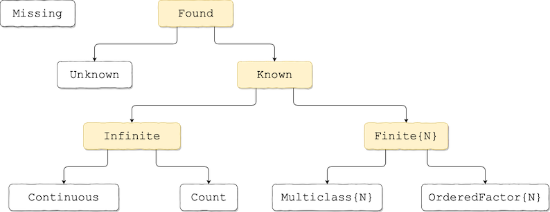
Figure 1. Part of the scientific type hierarchy in ScientificTypes.jl.

julia> scitype(4.6)
Continuous

julia> scitype(42)
Count

julia> x1 = categorical(["yes", "no", "yes", "maybe"]);

julia> scitype(x1)
AbstractArray{Multiclass{3},1}

julia> X = (x1=x1, x2=rand(4), x3=rand(4))  # a "column table"
(x1 = CategoricalValue{String,UInt32}["yes", "no", "yes", "maybe"],
 x2 = [0.6773327542735201, 0.7006103544430491, 0.08711892295263124, 0.10044148462265512],
 x3 = [0.7725728980157012, 0.4327687556359405, 0.47515672039406387, 0.8211160337597527],)

julia> scitype(X)
Table{Union{AbstractArray{Continuous,1}, AbstractArray{Multiclass{3},1}}}

Tabular data

All data containers compatible with the Tables.jl interface (which includes all source formats listed here) have the scientific type Table{K}, where K depends on the scientific types of the columns, which can be individually inspected using schema:

julia> schema(X)
┌─────────┬─────────────────────────────────┬───────────────┐
│ _.names │ _.types                         │ _.scitypes    │
├─────────┼─────────────────────────────────┼───────────────┤
│ x1      │ CategoricalValue{String,UInt32} │ Multiclass{3} │
│ x2      │ Float64                         │ Continuous    │
│ x3      │ Float64                         │ Continuous    │
└─────────┴─────────────────────────────────┴───────────────┘
_.nrows = 4

Inputs

Since an MLJ model only specifies the scientific type of data, if that type is Table - which is the case for the majority of MLJ models - then any Tables.jl format is permitted. However, the Tables.jl API excludes matrices. If Xmatrix is a matrix, convert it to a column table using X = MLJ.table(Xmatrix).

Specifically, the requirement for an arbitrary model's input is scitype(X) <: input_scitype(model).

Targets

The target y expected by MLJ models is generally an AbstractVector. A multivariate target y will generally be a table.

Specifically, the type requirement for a model target is scitype(y) <: target_scitype(model).

Querying a model for acceptable data types

Given a model instance, one can inspect the admissible scientific types of its input and target, and without loading the code defining the model:

julia> i = info("DecisionTreeClassifier")
CART decision tree classifier.
→ based on [DecisionTree](https://github.com/bensadeghi/DecisionTree.jl).
→ do `@load DecisionTreeClassifier pkg="DecisionTree"` to use the model.
→ do `?DecisionTreeClassifier` for documentation.
(name = "DecisionTreeClassifier",
 package_name = "DecisionTree",
 is_supervised = true,
 docstring = "CART decision tree classifier.\n→ based on [DecisionTree](https://github.com/bensadeghi/DecisionTree.jl).\n→ do `@load DecisionTreeClassifier pkg=\"DecisionTree\"` to use the model.\n→ do `?DecisionTreeClassifier` for documentation.",
 hyperparameter_ranges = (nothing, nothing, nothing, nothing, nothing, nothing, nothing, nothing, nothing),
 hyperparameter_types = ("Int64", "Int64", "Int64", "Float64", "Int64", "Bool", "Float64", "Float64", "Int64"),
 hyperparameters = (:max_depth, :min_samples_leaf, :min_samples_split, :min_purity_increase, :n_subfeatures, :post_prune, :merge_purity_threshold, :pdf_smoothing, :display_depth),
 implemented_methods = Symbol[:clean!, :fit, :fitted_params, :predict],
 is_pure_julia = true,
 is_wrapper = false,
 load_path = "MLJModels.DecisionTree_.DecisionTreeClassifier",
 package_license = "MIT",
 package_url = "https://github.com/bensadeghi/DecisionTree.jl",
 package_uuid = "7806a523-6efd-50cb-b5f6-3fa6f1930dbb",
 prediction_type = :probabilistic,
 supports_online = false,
 supports_weights = false,
 input_scitype = Table{_s23} where _s23<:Union{AbstractArray{_s25,1} where _s25<:Continuous, AbstractArray{_s25,1} where _s25<:Count, AbstractArray{_s25,1} where _s25<:OrderedFactor},
 target_scitype = AbstractArray{_s226,1} where _s226<:Finite,
 output_scitype = Unknown,)

julia> i.input_scitype
Table{_s23} where _s23<:Union{AbstractArray{_s25,1} where _s25<:Continuous, AbstractArray{_s25,1} where _s25<:Count, AbstractArray{_s25,1} where _s25<:OrderedFactor}

julia> i.target_scitype
AbstractArray{_s226,1} where _s226<:Finite

Container element types

Models in MLJ will always apply the MLJ convention described in MLJScientificTypes.jl to decide how to interpret the elements of your container types. Here are the key features of that convention:

• Any AbstractFloat is interpreted as Continuous.

• Any Integer is interpreted as Count.

• Any CategoricalValue or CategoricalString, x, is interpreted as Multiclass or OrderedFactor, depending on the value of x.pool.ordered.

• Strings and Chars are not interpreted as Multiclass or OrderedFactor (they have scitypes Textual and Unknown respectively).

• In particular, integers (including Bools) cannot be used to represent categorical data. Use the preceding coerce operations to coerce to a Finite scitype.

Use coerce(v, OrderedFactor) or coerce(v, Multiclass) to coerce a vector v of integers, strings or characters to a vector with an appropriate Finite (categorical) scitype. For more on scitype coercion of arrays and tables, see coerce, autotype and unpack below.

To designate an intrinsic "true" class for binary data (for purposes of applying MLJ measures, such as truepositive), data should be represented by an ordered CategoricalValue or CategoricalString. This data will have scitype OrderedFactor{2} and the "true" class is understood to be the second class in the ordering.

coerce(A, ...; tight=false, verbosity=1)

coerce(X, col1=>scitype1, col2=>scitype2, ... ; verbosity=1)
coerce(X, d::AbstractDict; verbosity=1)

using CategoricalArrays, DataFrames, Tables
X = DataFrame(name=["Siri", "Robo", "Alexa", "Cortana"],
              height=[152, missing, 148, 163],
              rating=[1, 5, 2, 1])
Xc = coerce(X, :name=>Multiclass, :height=>Continuous, :rating=>OrderedFactor)
schema(Xc).scitypes # (Multiclass, Continuous, OrderedFactor)

X  = (x = [1, 2, 3],
      y = rand(3),
      z = [10, 20, 30])
Xc = coerce(X, Count=>Continuous)
schema(Xfixed).scitypes # (Continuous, Continuous, Continuous)

autotype(X; kw...)

t1, t2, ...., tk = unnpack(table, f1, f2, ... fk;
                           wrap_singles=false,
                           shuffle=false,
                           rng::Union{AbstractRNG,Int}=nothing)

unpack(table, t...; wrap_singles=false, col1=>scitype1, col2=>scitype2, ... )

julia> table = DataFrame(x=[1,2], y=['a', 'b'], z=[10.0, 20.0], w=[:A, :B])
julia> Z, XY = unpack(table, ==(:z), !=(:w);
               :x=>Continuous, :y=>Multiclass)
julia> XY
2×2 DataFrame
│ Row │ x       │ y            │
│     │ Float64 │ Categorical… │
├─────┼─────────┼──────────────┤
│ 1   │ 1.0     │ 'a'          │
│ 2   │ 2.0     │ 'b'          │

julia> Z
2-element Array{Float64,1}:
 10.0
 20.0