Tuning models
In MLJ tuning is implemented as a model wrapper. After wrapping a model in a tuning strategy and binding the wrapped model to data in a machine, mach, calling fit!(mach) instigates a search for optimal model hyperparameters, within a specified range, and then uses all supplied data to train the best model. To predict using the optimal model, one just calls predict(mach, Xnew). In this way the wrapped model may be viewed as a "self-tuning" version of the unwrapped model.
Below we illustrate tuning by grid and random searches. For a complete list of available and planned tuning strategies, see the MLJTuning page
Tuning a single hyperparameter using a grid search
julia> using MLJ

julia> X = MLJ.table(rand(100, 10));

julia> y = 2X.x1 - X.x2 + 0.05*rand(100);

julia> tree_model = @load DecisionTreeRegressor;
Let's tune min_purity_increase in the model above, using a grid-search. To do so we will use the simplest range object, a one-dimensional range object constructed using the range method:
julia> r = range(tree_model, :min_purity_increase, lower=0.001, upper=1.0, scale=:log);

julia> self_tuning_tree_model = TunedModel(model=tree_model,
                                           resampling = CV(nfolds=3),
                                           tuning = Grid(resolution=10),
                                           range = r,
                                           measure = rms);
Incidentally, a grid is generated internally "over the range" by calling the iterator method with an appropriate resolution:
julia> iterator(r, 5)
5-element Array{Float64,1}:
 0.0010000000000000002
 0.005623413251903492
 0.0316227766016838
 0.1778279410038923
 1.0
Non-numeric hyperparameters are handled a little differently:
julia> selector_model = FeatureSelector();

julia> r2 = range(selector_model, :features, values = [[:x1,], [:x1, :x2]]);

julia> iterator(r2)
2-element Array{Array{Symbol,1},1}:
 [:x1]
 [:x1, :x2]
Unbounded ranges are also permitted. See the range and iterator docstrings below for details, and the sampler docstring for generating random samples from one-dimensional ranges (used internally by the RandomSearch strategy).
Returning to the wrapped tree model:
julia> self_tuning_tree = machine(self_tuning_tree_model, X, y);

julia> fit!(self_tuning_tree, verbosity=0);
We can inspect the detailed results of the grid search with report(self_tuning_tree) or just retrieve the optimal model, as here:
julia> fitted_params(self_tuning_tree).best_model
DecisionTreeRegressor(
    max_depth = -1,
    min_samples_leaf = 5,
    min_samples_split = 2,
    min_purity_increase = 0.0021544346900318843,
    n_subfeatures = 0,
    post_prune = false,
    merge_purity_threshold = 1.0) @616
Predicting on new input observations using the optimal model:
julia> Xnew  = MLJ.table(rand(3, 10));

julia> predict(self_tuning_tree, Xnew)
3-element Array{Float64,1}:
 0.1279048182145903
 0.5978222355696188
 0.20239883712432846
Tuning multiple nested hyperparameters
The following model has another model, namely a DecisionTreeRegressor, as a hyperparameter:
julia> tree_model = DecisionTreeRegressor()
julia> forest_model = EnsembleModel(atom=tree_model);
Ranges for nested hyperparameters are specified using dot syntax. In this case we will specify a goal for the total number of grid points:
julia> r1 = range(forest_model, :(atom.n_subfeatures), lower=1, upper=9);

julia> r2 = range(forest_model, :bagging_fraction, lower=0.4, upper=1.0);

julia> self_tuning_forest_model = TunedModel(model=forest_model,
                                             tuning=Grid(goal=30),
                                             resampling=CV(nfolds=6),
                                             range=[r1, r2],
                                             measure=rms);

julia> self_tuning_forest = machine(self_tuning_forest_model, X, y);

julia> fit!(self_tuning_forest, verbosity=0)
Machine{DeterministicTunedModel{Grid,…}} @940 trained 1 time.
  args:
    1:	Source @771 ⏎ `Table{AbstractArray{Continuous,1}}`
    2:	Source @073 ⏎ `AbstractArray{Continuous,1}`
In this two-parameter case, a plot of the grid search results is also available:
using Plots
plot(self_tuning_forest)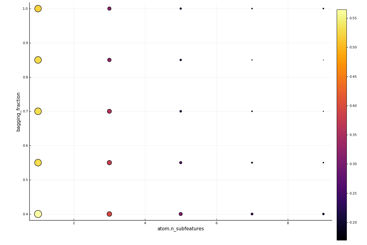
Instead of specifying a goal, we can declare a global resolution, which is overriden for a particular parameter by pairing it's range with the resolution desired. In the next example, the default resolution=100 is applied to the r2 field, but a resolution of 3 is applied to the r1 field. Additionally, we ask that the grid points be randomly traversed, and the the total number of evaluations be limited to 25.
julia> tuning = Grid(resolution=100, shuffle=true, rng=1234)
Grid(
    goal = nothing,
    resolution = 100,
    shuffle = true,
    rng = MersenneTwister(UInt32[0x000004d2]) @ 1002) @957

julia> self_tuning_forest_model = TunedModel(model=forest_model,
                                             tuning=tuning,
                                             resampling=CV(nfolds=6),
                                             range=[(r1, 3), r2],
                                             measure=rms,
                                             n=25);

julia> fit!(machine(self_tuning_forest_model, X, y), verbosity=0)
Machine{DeterministicTunedModel{Grid,…}} @011 trained 1 time.
  args:
    1:	Source @236 ⏎ `Table{AbstractArray{Continuous,1}}`
    2:	Source @603 ⏎ `AbstractArray{Continuous,1}`
For more options for a grid search, see Grid below.
Tuning using a random search
Let's attempt to tune the same hyperparameters using a RandomSearch tuning strategy. By default, bounded numeric ranges like r1 and r2 are sampled uniformly (before rounding, in the case of the integer range r1). Positive unbounded ranges are sampled using a Gamma distribution by default, and all others using a (truncated) normal distribution.
julia> self_tuning_forest_model = TunedModel(model=forest_model,
                                             tuning=RandomSearch(),
                                             resampling=CV(nfolds=6),
                                             range=[r1, r2],
                                             measure=rms,
                                             n=25);

julia> self_tuning_forest = machine(self_tuning_forest_model, X, y);

julia> fit!(self_tuning_forest, verbosity=0)
Machine{DeterministicTunedModel{RandomSearch,…}} @165 trained 1 time.
  args:
    1:	Source @810 ⏎ `Table{AbstractArray{Continuous,1}}`
    2:	Source @118 ⏎ `AbstractArray{Continuous,1}`
using Plots
plot(self_tuning_forest)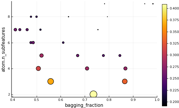
The prior distributions used for sampling each hyperparameter can be customized, as can the global fallbacks. See the RandomSearch doc-string below for details.
API
Base.range — Functionr = range(model, :hyper; values=nothing)Define a one-dimensional NominalRange object for a field hyper of model. Note that r is not directly iterable but iterator(r) is.
By default, the behaviour of range methods depends on the type of the value of the hyperparameter :hyper at model during range construction.
To override this behaviour (for instance if model is not available) specify a type in place of model so the behaviour depends on the value of the specified type.
A nested hyperparameter is specified using dot notation. For example, :(atom.max_depth) specifies the max_depth hyperparameter of the submodel model.atom.
r = range(model, :hyper; upper=nothing, lower=nothing,
          scale=nothing, values=nothing)
Assuming values is not specified, defines a one-dimensional NumericRange object for a Real field hyper of model. Note that r is not directly iteratable but iterator(r, n)is an iterator of length n. To generate random elements from r, instead apply rand methods to sampler(r). The supported scales are :linear,:log, :logminus, :log10, :log2, or a callable object.
A nested hyperparameter is specified using dot notation (see above).
If scale is unspecified, it is set to :linear, :log, :logminus, or :linear, according to whether the interval (lower, upper) is bounded, right-unbounded, left-unbounded, or doubly unbounded, respectively. Note upper=Inf and lower=-Inf are allowed.
If values is specified, the other keyword arguments are ignored and a NominalRange object is returned (see above).
MLJBase.iterator — Functioniterator([rng, ], r::NominalRange, [,n])
iterator([rng, ], r::NumericRange, n)Return an iterator (currently a vector) for a ParamRange object r. In the first case iteration is over all values stored in the range (or just the first n, if n is specified). In the second case, the iteration is over approximately n ordered values, generated as follows:
(i) First, exactly n values are generated between U and L, with a spacing determined by r.scale (uniform if scale=:linear) where U and L are given by the following table:
r.lower | r.upper | L | U |
|---|---|---|---|
| finite | finite | r.lower | r.upper |
-Inf | finite | r.upper - 2r.unit | r.upper |
| finite | Inf | r.lower | r.lower + 2r.unit |
-Inf | Inf | r.origin - r.unit | r.origin + r.unit |
(ii) If a callable f is provided as scale, then a uniform spacing is always applied in (i) but f is broadcast over the results. (Unlike ordinary scales, this alters the effective range of values generated, instead of just altering the spacing.)
(iii) If r is a discrete numeric range (r isa NumericRange{<:Integer}) then the values are additionally rounded, with any duplicate values removed. Otherwise all the values are used (and there are exacltly n of them).
(iv) Finally, if a random number generator rng is specified, then the values are returned in random order (sampling without replacement), and otherwise they are returned in numeric order, or in the order provided to the range constructor, in the case of a NominalRange.
Distributions.sampler — Functionsampler(r::NominalRange, probs::AbstractVector{<:Real})
sampler(r::NominalRange)
sampler(r::NumericRange{T}, d)Construct an object s which can be used to generate random samples from a ParamRange object r (a one-dimensional range) using one of the following calls:
rand(s)             # for one sample
rand(s, n)          # for n samples
rand(rng, s [, n])  # to specify an RNG
The argument probs can be any probability vector with the same length as r.values. The second sampler method above calls the first with a uniform probs vector.
The argument d can be either an arbitrary instance of UnivariateDistribution from the Distributions.jl package, or one of a Distributions.jl types for which fit(d, ::NumericRange) is defined. These include: Arcsine, Uniform, Biweight, Cosine, Epanechnikov, SymTriangularDist, Triweight, Normal, Gamma, InverseGaussian, Logistic, LogNormal, Cauchy, Gumbel, Laplace, and Poisson; but see the doc-string for Distributions.fit for an up-to-date list.
If d is an instance, then sampling is from a truncated form of the supplied distribution d, the truncation bounds being r.lower and r.upper (the attributes r.origin and r.unit attributes are ignored). For discrete numeric ranges (T <: Integer) the samples are rounded.
If d is a type then a suitably truncated distribution is automatically generated using Distributions.fit(d, r).
Important. Values are generated with no regard to r.scale, except in the special case r.scale is a callable object f. In that case, f is applied to all values generated by rand as described above (prior to rounding, in the case of discrete numeric ranges).
Examples
r = range(Char, :letter, values=collect("abc"))
s = sampler(r, [0.1, 0.2, 0.7])
samples =  rand(s, 1000);
StatsBase.countmap(samples)
Dict{Char,Int64} with 3 entries:
  'a' => 107
  'b' => 205
  'c' => 688

r = range(Int, :k, lower=2, upper=6) # numeric but discrete
s = sampler(r, Normal)
samples = rand(s, 1000);
UnicodePlots.histogram(samples)
           ┌                                        ┐
[2.0, 2.5) ┤▇▇▇▇▇▇▇▇▇▇▇▇▇▇ 119
[2.5, 3.0) ┤ 0
[3.0, 3.5) ┤▇▇▇▇▇▇▇▇▇▇▇▇▇▇▇▇▇▇▇▇▇▇▇▇▇▇▇▇▇▇▇▇▇▇▇ 296
[3.5, 4.0) ┤ 0
[4.0, 4.5) ┤▇▇▇▇▇▇▇▇▇▇▇▇▇▇▇▇▇▇▇▇▇▇▇▇▇▇▇▇▇▇▇▇▇ 275
[4.5, 5.0) ┤ 0
[5.0, 5.5) ┤▇▇▇▇▇▇▇▇▇▇▇▇▇▇▇▇▇▇▇▇▇▇▇▇▇▇ 221
[5.5, 6.0) ┤ 0
[6.0, 6.5) ┤▇▇▇▇▇▇▇▇▇▇▇ 89
           └                                        ┘
StatsBase.fit — MethodDistributions.fit(D, r::MLJBase.NumericRange)Fit and return a distribution d of type D to the one-dimensional range r.
Only types D in the table below are supported.
The distribution d is constructed in two stages. First, a distributon d0, characterized by the conditions in the second column of the table, is fit to r. Then d0 is truncated between r.lower and r.upper to obtain d.
Distribution type D | Characterization of d0 |
|---|---|
Arcsine, Uniform, Biweight, Cosine, Epanechnikov, SymTriangularDist, Triweight | minimum(d) = r.lower, maximum(d) = r.upper |
Normal, Gamma, InverseGaussian, Logistic, LogNormal | mean(d) = r.origin, std(d) = r.unit |
Cauchy, Gumbel, Laplace, (Normal) | Dist.location(d) = r.origin, Dist.scale(d) = r.unit |
Poisson | Dist.mean(d) = r.unit |
Here Dist = Distributions.
MLJTuning.TunedModel — Functiontuned_model = TunedModel(; model=nothing,
tuning=Grid(),
resampling=Holdout(),
measure=nothing,
weights=nothing,
repeats=1,
operation=predict,
range=nothing,
n=default_n(tuning, range),
train_best=true,
acceleration=default_resource(),
acceleration_resampling=CPU1(),
check_measure=true)Construct a model wrapper for hyperparameter optimization of a supervised learner.
Calling fit!(mach) on a machine mach=machine(tuned_model, X, y) or mach=machine(tuned_model, X, y, w) will:
Instigate a search, over clones of
model, with the hyperparameter mutations specified byrange, for a model optimizing the specifiedmeasure, using performance evaluations carried out using the specifiedtuningstrategy andresamplingstrategy.Fit an internal machine, based on the optimal model
fitted_params(mach).best_model, wrapping the optimalmodelobject in all the provided dataX,y(,w). Callingpredict(mach, Xnew)then returns predictions onXnewof this internal machine. The final train can be supressed by settingtrain_best=false.
The range objects supported depend on the tuning strategy specified. Query the strategy docstring for details. To optimize over an explicit list v of models of the same type, use strategy=Explicit() and specify model=v[1] and range=v.
The number of models searched is specified by n. If unspecified, then MLJTuning.default_n(tuning, range) is used. When n is increased and fit!(mach) called again, the old search history is re-instated and the search continues where it left off.
If measure supports weights (supports_weights(measure) == true) then any weights specified will be passed to the measure. If more than one measure is specified, then only the first is optimized (unless strategy is multi-objective) but the performance against every measure specified will be computed and reported in report(mach).best_performance and other relevant attributes of the generated report.
Specify repeats > 1 for repeated resampling per model evaluation. See evaluate! options for details.
Important. If a custom measure is used, and the measure is a score, rather than a loss, be sure to check that MLJ.orientation(measure) == :score to ensure maximization of the measure, rather than minimization. Override an incorrect value with MLJ.orientation(::typeof(measure)) = :score.
Important: If weights are left unspecified, and measure supports sample weights, then any weight vector w used in constructing a corresponding tuning machine, as in tuning_machine = machine(tuned_model, X, y, w) (which is then used in training each model in the search) will also be passed to measure for evaluation.
In the case of two-parameter tuning, a Plots.jl plot of performance estimates is returned by plot(mach) or heatmap(mach).
Once a tuning machine mach has bee trained as above, then fitted_params(mach) has these keys/values: key | value ––––––––––|––––––––––––––––––––––––– best_model | optimal model instance best_fitted_params| learned parameters of the optimal model The named tuple report(mach) includes these keys/values: key | value ––––––––––|––––––––––––––––––––––––– best_model | optimal model instance best_result | corresponding "result" entry in the history best_report | report generated by fitting the optimal model history | tuning strategy-specific history of all evaluations plus others specific to the tuning strategy, such as history=....
Summary of key-word arguments
model:Supervisedmodel prototype that is cloned and mutated to generate models for evaluationtuning=Grid(): tuning strategy to be applied (eg,RandomSearch())resampling=Holdout(): resampling strategy (eg,Holdout(),CV()),StratifiedCV()) to be applied in performance evaluationsmeasure: measure or measures to be applied in performance evaluations; only the first used in optimization (unless the strategy is multi-objective) but all reported to the historyweights: sample weights to be passed the measure(s) in performance evaluations, if supported (see important note above for behaviour in unspecified case)repeats=1: for generating train/test sets multiple times in resampling; seeevaluate!for detailsoperation=predict: operation to be applied to each fitted model; usuallypredictbutpredict_mean,predict_medianorpredict_modecan be used forProbabilisticmodels, if the specified measures areDeterministicrange: range object; tuning strategy documentation describes supported typesn: number of iterations (ie, models to be evaluated); set by tuning strategy if left unspecifiedtrain_best=true: whether to train the optimal modelacceleration=default_resource(): mode of parallelization for tuning strategies that support thisacceleration_resampling=CPU1(): mode of parallelization for resamplingcheck_measure: whether to checkmeasureis compatible with the specifiedmodelandoperation)
MLJTuning.Grid — TypeGrid(goal=nothing, resolution=10, rng=Random.GLOBAL_RNG, shuffle=true)Instantiate a Cartesian grid-based hyperparameter tuning strategy with a specified number of grid points as goal, or using a specified default resolution in each numeric dimension.
Supported ranges:
A single one-dimensional range or vector of one-dimensioinal ranges can be specified. Specifically, in Grid search, the range field of a TunedModel instance can be:
A single one-dimensional range - ie,
ParamRangeobject -r, or pair of the form(r, res)whereresspecifies a resolution to override the defaultresolution.Any vector of objects of the above form
Two elements of a range vector may share the same field attribute, with the effect that their grids are combined, as in Example 3 below.
ParamRange objects are constructed using the range method.
Example 1:
range(model, :hyper1, lower=1, origin=2, unit=1)Example 2:
[(range(model, :hyper1, lower=1, upper=10), 15),
  range(model, :hyper2, lower=2, upper=4),
  range(model, :hyper3, values=[:ball, :tree])]
Example 3:
# a range generating the grid `[1, 2, 10, 20, 30]` for `:hyper1`:
[range(model, :hyper1, values=[1, 2]),
 (range(model, :hyper1, lower= 10, upper=30), 3)]
Note: All the field values of the ParamRange objects (:hyper1, :hyper2, :hyper3 in the preceding example) must refer to field names a of single model (the model specified during TunedModel construction).
Algorithm
This is a standard grid search with the following specifics: In all cases all values of each specified NominalRange are exhausted. If goal is specified, then all resolutions are ignored, and a global resolution is applied to the NumericRange objects that maximizes the number of grid points, subject to the restriction that this not exceed goal. (This assumes no field appears twice in the range vector.) Otherwise the default resolution and any parameter-specific resolutions apply.
In all cases the models generated are shuffled using rng, unless shuffle=false.
See also TunedModel, range.
MLJTuning.RandomSearch — TypeRandomSearch(bounded=Distributions.Uniform,
positive_unbounded=Distributions.Gamma,
other=Distributions.Normal,
rng=Random.GLOBAL_RNG)Instantiate a random search tuning strategy, for searching over Cartesian hyperparameter domains, with customizable priors in each dimension.
Supported ranges
A single one-dimensional range or vector of one-dimensioinal ranges can be specified. If not paired with a prior, then one is fitted, according to fallback distribution types specified by the tuning strategy hyperparameters. Specifically, in RandomSearch, the range field of a TunedModel instance can be:
a single one-dimensional range (
ParamRangeobject)ra pair of the form
(r, d), withras above and wheredis:a probability vector of the same length as
r.values(raNominalRange)any
Distributions.UnivariateDistributioninstance (raNumericRange)one of the subtypes of
Distributions.UnivariateDistributionlisted in the table below, for automatic fitting usingDistributions.fit(d, r), a distribution whose support always lies betweenr.lowerandr.upper(raNumericRange)
any pair of the form
(field, s), wherefieldis the (possibly nested) name of a field of the model to be tuned, andsan arbitrary sampler object for that field. This means only thatrand(rng, s)is defined and returns valid values for the field.any vector of objects of the above form
A range vector may contain multiple entries for the same model field, as in range = [(:lambda, s1), (:alpha, s), (:lambda, s2)]. In that case the entry used in each iteration is random.
| distribution types | for fitting to ranges of this type |
|---|---|
Arcsine, Uniform, Biweight, Cosine, Epanechnikov, SymTriangularDist, Triweight | bounded |
Gamma, InverseGaussian, Poisson | positive (bounded or unbounded) |
Normal, Logistic, LogNormal, Cauchy, Gumbel, Laplace | any |
ParamRange objects are constructed using the range method.
Examples
using Distributions

range1 = range(model, :hyper1, lower=0, upper=1)

range2 = [(range(model, :hyper1, lower=1, upper=10), Arcsine),
          range(model, :hyper2, lower=2, upper=Inf, unit=1, origin=3),
          (range(model, :hyper2, lower=2, upper=4), Normal(0, 3)),
          (range(model, :hyper3, values=[:ball, :tree]), [0.3, 0.7])]

# uniform sampling of :(atom.λ) from [0, 1] without defining a NumericRange:
struct MySampler end
Base.rand(rng::Random.AbstractRNG, ::MySampler) = rand(rng)
range3 = (:(atom.λ), MySampler())
Algorithm
In each iteration, a model is generated for evaluation by mutating the fields of a deep copy of model. The range vector is shuffled and the fields sampled according to the new order (repeated fields being mutated more than once). For a range entry of the form (field, s) the algorithm calls rand(rng, s) and mutates the field field of the model clone to have this value. For an entry of the form (r, d), s is substituted with sampler(r, d). If no d is specified, then sampling is uniform (with replacement) if r is a NominalRange, and is otherwise given by the defaults specified by the tuning strategy parameters bounded, positive_unbounded, and other, depending on the field values of the NumericRange object r.
See also TunedModel, range, sampler.