1. Introduction
TATi contains a set of distinct guides aimed at different user audiences. All of them reside in <installation folder>/share/doc/thermodynamicanalyticstoolkit/ in the installation folder.
-
User guide (this document: userguide.html or userguide.pdf)
-
Programmer’s guide (see programmersguide.html or programmersguide.pdf)
-
Reference documentation (see thermodynamicanalyticstoolkit-API-reference.pdf or html/index.html)
-
Roadmap (see roadmap.html or roadmap.pdf)
1.1. Before you start
In the following we assume that you, the reader, has a general familiarity with neural networks. You should know what a classification problem is, what an associated dataset for (supervised) learning needs to contain. You should know about what weights and biases in a neural network are and what the loss function does. You should also have a rough idea of what optimization is and that gradients with respect to the chosen loss function can be obtained through so-called backpropagation.
If you are not familiar with the above terminology, then we recommend an introductory book on neural networks such as [Bishop2006].
1.2. What is ThermodynamicAnalyticsToolkit?
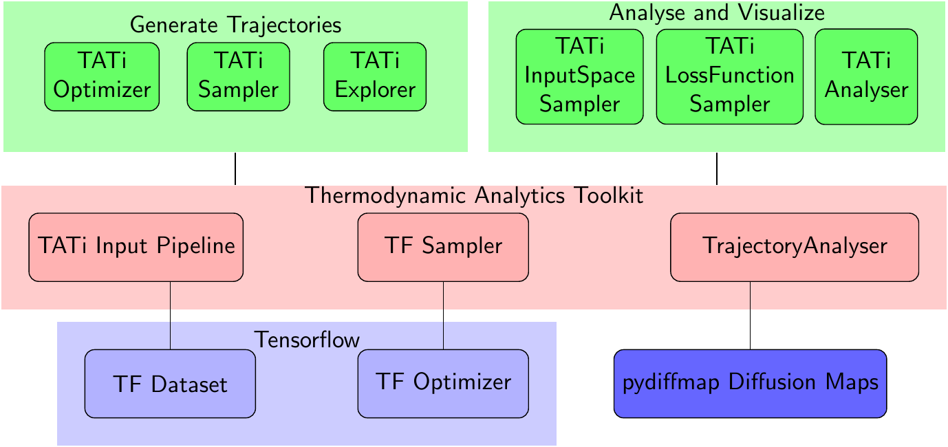
The Thermodynamic Analytics Toolkit allows to perform thermodynamic sampling and analysis of large neural network loss manifolds. It extends Tensorflow by several samplers, by a framework to rapidly prototype new samplers, by the capability to sample several networks in parallel and provides tools for analysis and visualization of loss manifolds, see Figure [introduction.figure.tools_module] for an overview. We rely on the Python programming language as only for that Tensorflow’s interface has an API stability promise.
There are two approaches to using TATi: On the one hand, it is a toolkit consisting of command-line programs such as TATiOptimizer, TATiSampler, TATiLossFunctionSampler, and TATiAnalyzer that, when fed a dataset and given the network specifics, directly allow to optimize and sample the network parameters and analyze the exlored loss manifold, see Figure [introduction.figure.tools_module].
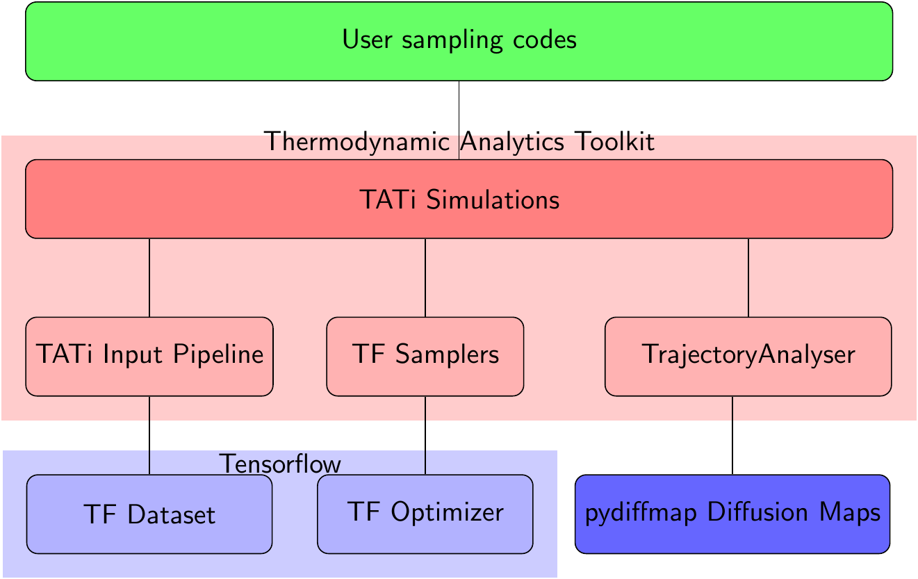
On the other hand, TATi can be readily used inside Python programs by using its modules: simulation, model, analysis. The simulation module, see Figure [introduction.figure.simulation_module], contains a very easy-to-use, high-level interface to neural network modelling, granting full access to the network’s parameters, its gradients, its loss and all other quantities of interest. It is especially practical for rapid prototyping. The module model is its low-level counterpart and allows for more efficient implementations.
Beginning with section [quickstart] we give an introduction to either way of using TATi.
1.3. Installation
In the following we explain the installation procedure to get ThermodynamicAnalyticsToolkit up and running.
The easiest way to tati is through ```` pip install tati ````
If you want to install from a cloned repository or from a release tarball, then read on.
1.3.1. Installation requirements
This program suite is implemented using python3 and the development mainly focused on Linux (development machine used Ubuntu 14.04 up to 18.04). At the moment other operating systems are not supported but may still work.
It has the following non-trivial dependencies:
-
TensorFlow: version 1.4.1 till currently 1.10 supported
Note that these packages can be easily installed using either the repository tool (using some linux derivate such as Ubuntu), e.g.
sudo apt install python3-numpy
or via pip3, i.e.
pip3 install numpy
For acor a few extra changes are required.
pip3 install acor
sed -i -e "s#import _acor#import acor._acor as _acor#" <install path>/acor/acor.py
The last command replaces the third line in the file acor/acor.py such that the function acor (and not the module acor) is used.
|
Note
|
acor is only required for the Integrated Autocorrelation Time analysis and may be ignored if this functionality is not required. |
Moreover, the following packages are not ultimately required but examples or tests may depend on them:
-
gawk
The documentation is written in AsciiDoc and doxygen and requires a suitable package to compile to HTML or create a PDF, e.g., using dblatex
-
doxygen
-
asciidoc
-
dblatex
Finally, for the diffusion map analysis we recommend using the pydiffmap package, see https://github.com/DiffusionMapsAcademics/pyDiffMap.
In our setting what typically worked best was to use anaconda in the following manner:
conda create -n tensorflow python=3.5 -y
conda install -n tensorflow -y \
     tensorflow numpy scipy pandas scikit-learn matplotlib
In case your machine has GPU hardware for tensorflow, replace “tensorflow” by “tensorflow-gpu”.
|
Note
|
On systems with typical core i7 architecture recompiling tensorflow from source provided only very small runtime gains in our tests which in most cases do not support the extra effort. You may find it necessary for tackling really large networks (>1e6 dofs) and datasets and especially if you desire to use Intel’s MKL library for the CPU-based linear algebra computations. |
|
Tip
|
acor cannot be installed using anaconda (not available). Hence, it needs to be installed using pip for the respective environment. See above for installation instructions. |
Henceforth, we assume that there is a working tensorflow on your system, i.e. inside the python3 shell
import tensorflow as tf

a=tf.constant("Hello world")
sess=tf.Session()
print(sess.run(a))
should print “Hello world” or similar.
|
Tip
|
You can check the version of your tensorflow installation at any time by inspecting print(tf.__version__). Similarly, TATi’s version can be obtained through import TATi print(TATi.__version__) |
1.3.2. Installation procedure
Installation comes in three flavors: as a PyPI package, or through either via a tarball or a cloned repository.
In general, the PyPI (pip) packages are strongly recommended, especially if you only want to use the software.
The tarball releases are recommended if you only plan to use TATi and do not intend ito modify its code. If, however, you need to use a development branch, then you have to clone from the repository.
In general, this package is distributed via autotools, "compiled" and installed via automake. If you are familiar with this set of tools, there should be no problem. If not, please refer to the text INSTALL file that is included in the tarball.
|
Note
|
Only the tarball contains precompiled PDFs of the userguides. The cloned repository contains only the HTML pages. |
1.3.3. From Tarball
Unpack the archive, assuming its suffix is .bz2.
tar -jxvf thermodynamicanalyticstoolkit-${revnumber}.tar.bz2
If the ending is .gz, you need to unpack by
tar -zxvf thermodynamicanalyticstoolkit-${revnumber}.tar.gz
Enter the directory
cd thermodynamicanalyticstoolkit
Continue then in section Configure, make, install.
1.3.4. From cloned repository
While the tarball does not require any autotools packages installed on your system, the cloned repository does. You need the following packages:
-
autotools
-
automake
To prepare code in the working directory, enter
./bootstrap.sh
1.3.5. Configure, make, make install
Next, we recommend to build the toolkit not in the source folder but in an extra folder, e.g., “build64”. In the autotools lingo this is called an out-of-source build. It prevents cluttering of the source folder. Naturally, you may pick any name (and actually any location on your computer) as you see fit.
mkdir build64
cd build64
../configure --prefix="somepath" -C PYTHON="path to python3"
make
make install
More importantly, please replace “somepath” and “path to python3” by the desired installation path and the full path to the python3 executable on your system.
|
Note
|
In case of having used anaconda for the installation of required packages, then you need to use $HOME/.conda/envs/tensorflow/bin/python3 for the respective command, where $HOME is your home folder. This assumes that your anaconda environment is named tensorflow as in the example installation steps above. |
|
Note
|
We recommend executing (after make install was run) make -j4 check additionally. This will execute every test on the extensive testsuite and report any errors. None should fail. If all fail, a possible cause might be a not working tensorflow installation. If some fail, please contact the author. The extra argument -j4 instructs make to use four threads in parallel for testing. Use as many as you have cores on your machine. In case you run the testcases on strongly parallel hardware, tests may fail because of cancellation effects during parallel summation. In this case you made degrade the test threshold using the environment variable TATI_TEST_THRESHOLD. If unset, it defaults to 1e-7. |
|
Tip
|
Tests may fail due to numerical inaccuracies due to reduction operations executed in parallel. Tensorflow does not emphasize on determinism but on speed and scaling. Therefore, if your system has many cores or is GPU-assisted, some tests may fail. In this case you can set the environment variable TATI_TEST_THRESHOLD when calling configure. Its default value is 1e-7. For the DGX-1 we found 4e-6 to work. If the threshold need to run all test successfully is much larger than this, you should contact us, see [introduction.feedback]. |
1.4. License
As long as no other license statement is given, ThermodynamicAnalyticsToolkit is free for use under the GNU Public License (GPL) Version 3 (see https://www.gnu.org/licenses/gpl-3.0.en.html for full text).
1.5. Disclaimer
Because the program is licensed free of charge, there is not warranty for the program, to the extent permitted by applicable law. Except when otherwise stated in writing in the copyright holders and/or other parties provide the program "as is" without warranty of any kind, either expressed or implied. Including, but not limited to, the implied warranties of merchantability and fitness for a particular purpose. The entire risk as to the quality and performance of the program is with you. Should the program prove defective, you assume the cost of all necessary servicing, repair, or correction.
— section 11 of the GPLv3 license
1.6. Feedback
If you encounter any bugs, errors, or would like to submit feature request, please open an issue at GitHub or write to frederik.heber@gmail.com. The authors are especially thankful for any description of all related events prior to occurrence of the error and auxiliary files. More explicitly, the following information is crucial in enabling assistance:
-
operating system and version, e.g., Ubuntu 16.04
-
Tensorflow version, e.g., TF 1.6
-
TATi version (or respective branch on GitHub), e.g., TATi 0.8
-
steps that lead to the error, possibly with sample Python code
Please mind sensible space restrictions of email attachments.
2. Quickstart
Before we come to actually using TATi, we explain what possible approaches there are to sampling a high-dimensional function such as the loss manifold of neural networks. To this end, we talk about grid-based sampling that however suffers from the Curse of Dimensionality. Moreover, we will discuss Monte Carlo and especially Markov Chain Monte Carlo methods. In the latter category we have what we will call dynamics-based sampling. This approach does not suffer in principle from the Curse of Dimensionality but moreover may have additional savings by looking only at areas of the manifold that have small loss. At the end, want to set the stage with a little example: We will look at a very simple classification task and see how it is solved using neural networks.
2.1. Sampling
Let be given a high-dimensional loss manifold
$L_{D}(\theta) = \sum_{(x_i,y_i) \in {D}} l_\theta(x_i,y_i)$
that depends explicitly on the parameters $\theta \in \Omega \subset \mathrm{R}^N$ of the network with $N$ degrees of freedom and implicitly on a given dataset ${D} = \{x_i,y_i\}$. Furthermore, the loss function $l_\theta$ itself depends implicitly on the prediction $f_\theta(x_i)$ of the network for a given input $x_i$ and fixed parameters $\theta$ and therefore on the chosen network architecture.
If ${D}$ were the set of all possible realisations of the data, then $L_{D}(\theta)$ would measure the so-called generalization error. As typically only a finite set of data is available, it is split into training and test parts, the latter set aside for approximating this error. Furthermore, during training the gradient is often computed on a subset of the training set ${D}$, the mini-batches. In the following we will ignore these details as they are irrelevant to the general procedure described.
In order to deduce information such as the number of minima, the number of saddle points, the typical barrier height between minima and other characteristics to classify the landscape, we need to explore the whole domain $\Omega$. As $L_{D}$ depends on an arbitrary dataset, we do not know anything a-priori apart from the general regularity properties
[As activation functions contained in the loss may be non-smooth, e.g., the rectified linear unit, even this can be not taken as solid grounds.]
and possible boundedness of $l_\theta$.
A very similar task is found in function approximation where an unknown and possibly high-dimensional function $f(x): \mathrm{R}^N \rightarrow \mathrm{R}$ is approximated through a set of point evaluations in conjunction with a basis set. A typical usecase is the numerical integration of this high-dimensional function. Naturally, the quality of the approximation hinges not only on the basis set but even more on the choice of the precise location of point evaluations, the sampling.
Very generally, sampling approaches can be placed into two categories: Grids and sequences. Sequences can be random, deterministic, or both. We briefly discuss them, focusing on their general computational cost in high dimensions.
2.1.1. Grids
Structured grids such as naive full grid approaches, where a fixed number of points with equidistant spacing is used per axis, suffer from the Curse of Dimensionality, a term coined by Bellman. With increasing number of parameters $N$ the computational cost becomes prohibitive. This Curse of Dimensionality is alleviated to some extent by so-called Sparse Grids, see [Bungartz2004], where the quality bounds on the approximation are kept but fewer grid points need to be evaluated. However, they only alleviate the curse to some extent, see [Pflueger2010], and are still infeasible at the moment for the extremely high-dimensional manifolds encountered in neural network losses.
2.1.2. Sequences
Random sequences are Monte Carlo approaches where a specific sequence of random numbers decides which point in the whole space to evaluate. Due to their inherent stochasticity these lack the rigor of the structured grid methods but neither rely on, nor exploit any regularity as the structured grid methods. Therefore, they suffer no Curse of Dimensionality with respect to their convergence rate. The rate is bounded by the Central Limit Theorem to ${O}(n^{-\frac 1 2})$ if $n$ is the number of evaluated points.
Quasi-Monte Carlo (QMC) methods use deterministic sequences, such as Lattice rules (Hammersley, \ldots) or digital nets, and are able to obtain higher convergence rates of ${O}(n^{-1} (\log{n})^d)$ at the price of a moderate dependence on dimension $d$.
In this category of sequences we also have dynamics-based sequences. As examples of Markov Chain Monte Carlo (MCMC) methods, they are closely connected to pure Monte Carlo approaches. They make use of the ergodic property of the chosen dynamics allowing to replace high-dimensional whole-space integrals by single-dimensional time-integrals, where the accuracy depends on the trajectory length.
The chain can be generated through suitable dynamics such as Hamiltonian,
$d\theta= M^{-1} p dt, \quad dp= -\nabla L(\theta) dt$
or Langevin dynamics,
$d\theta= M^{-1} p dt, \quad dp= \Bigl (-\nabla L(\theta) - \gamma p \Bigr ) dt + \sigma M^{\frac 1 2} dW$
for positions (or parameters) $\theta$, momenta $p$, mass matrix $M$, potential (or loss) $L(\theta)$, friction constant $\gamma$ and a stationary normal random process $W$ with variance $\sigma$. Note that Langevin dynamics has both Hamiltonian dynamics and Brownian dynamics as limiting cases of the friction constant $\gamma$ going to zero or infinity, respectively.
There are also hybrid approaches where a purely deterministic sequence is randomized by a Metropolis-Hastings criterion to remove possible bias, such as Hybrid or Hamiltonian Monte Carlo, see [Neal2011]. Note that in the case of Langevin dynamics the stochasticity enters through the random process.
If we consider the function $L_{D}(\theta)$ as a potential energy function, then we may cast this into a probability distribution using the canonical Gibbs distribution $Z \cdot \exp( -\beta L_{D}(\theta))$, where $Z$ is a normalization constant and $\beta$ is the inverse temperature factor. Then, we have sampling in the typical sense in statistics where an unknown distribution is evaluated. We remark that this Gibbs measure is known in the neural networks community through the energy interpretation ([LeCun2006) of a probability distribution in relation to a certain reference energy, given by the temperature.
And indeed, dynamics-based sampling does not aim to approximate $L$ as best as possible but its Gibbs (also called the canonical) distribution $\exp{(-\beta L)}$. In our case we are only interested in particular subsets of the space, namely those associated with a small loss. As we have given ample evidence, the central challenge in sampling is the computational cost. The dynamics-based sequences allow to save computational cost in the high-dimensional spaces by incorporating gradient information. Hence, the more accurately we sample from the Gibbs distribution, the more efficiently we sample only those subsets of interest. This saving could not be obtained with a pure Monte Carlo approach.
Therefore, we focus on dynamics-based sampling for this high-dimensional exploration problem.
2.1.3. Integrated Autocorrelation Time
In principle, the underlying challenge is to assure that the sampling trajectory covers a sufficient area of the whole space for validity. However, stating when to terminate is as difficult as the exploration task itself. Hence, the best measure is to assess when a new independent state has been obtained.
When inspecting sampled MCMC trajectories, we need to assess how many consecutive steps it takes to get from one independent state to another. This is estimated by the Integrated Autocorrelation Time (IAT) $\tau_s$. For any observable $A$, we have that its variance generally behaves as $var_{A} = \frac {var_{\pi} (\varphi(X))}{T_s/\tau_s}$, where $\pi$ is the target density, $\varphi(X)$ is the function of interest of the random variable $X$, and $T_s$ is the sampling time, see [Goodman2010]. Obviously, when time steps are discrete and $\tau_s$ is measured in number of steps, then $\tau_s = 1$ is highly desirable, i. e.~immediately stepping from one independent state to the next. The IAT $\tau_s$ is defined as
$\tau_s = \sum^{\infty}_{-\infty} \frac{ C_s(t)} {C_s(0)} \quad {with} \quad C_s(t) = \lim_{t' \rightarrow \infty} cov[\varphi \bigl (X(t'+t) \bigr ), \varphi \bigl (X(t) \bigr)$].
The above holds also for sampling approaches based on Langevin Dynamics. There, we may use the IAT to gauge the exploration speed for each sampled trajectory $X(t)$.
2.1.4. Example: Sampling of a Perceptron
Let us give a trivial example to illustrate the above with a few figures. We want to highlight in the following the key aspect about the dynamics-based sampling approach, namely sampling the probability distribution function associated with the Gibbs measure and not the loss manifold directly.
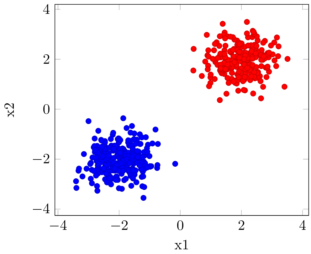
Assume we are given a very simple data set as depicted in Dataset. The goal is to classify all red and blue dots into two different classes. This problem is quite simple to solve: a line in the two-dimensional space can easily separate the two classes.
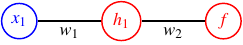
A very simple neural network, a perceptron: it would use one input node, either of the coordinate, $x_{1}$ or $x_{2}$, and a single output node with an activation function $f$ whose sign gives the class the input item belongs to. The network is given in Network. The network is chosen non-ideal by design to illustrate a point.
In Figure Loss manifold we then turn to the two-dimensional loss landscape depending on the two weights. In this very low-dimensional case we turn to the "naive grid" approach and partition each axis equidistantly. We see two minima basins both of hyperbole or "banana" shape. Here, we see that there is not a single minima but two of them. This is caused by the deliberate permutation symmetry of the two weights in the network.
Assume we additionally perform dynamics-based sampling. In the figure the resulting trajectory is given as squiggly black line. Here, we have chosen such an (inverse) temperature value such that it is able to pass the potential barrier and reach the other minima basin.
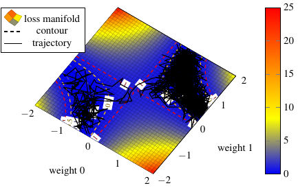
As we clearly see, the grid-based approach does not distinguish between the areas of high loss and the areas of low loss. Note that the coloring comes from a spline interpolation from the grid points. The dynamics-based trajectory on the other hand remains in areas of low loss all the time, where "low" is relative to its inverse temperature parameter. This is because the areas of low loss have a much higher probability in the Gibbs measure which our sampler is faithful to.
This quick description of the sampling loss manifolds in the context of neural networks in data science should have acquainted we with some of the concepts underlying the idea of sampling.
2.2. Using module simulation
The simulation module has been designed explicitly for ease-of-use. Typically, everything is achieved through two or three commands: One to setup TATi by handing it a dash of options, then calling a function to fit() or sample(). In the very end of this quickstart we will learn how to implement our first sampler using this interface.
For a more extensive description of the simulation module, we refer to its reference section.
If we have installed the TATi package in the folder /foo, i.e. we have a folder TATi with a file simulation.py residing in there, then we probably need to add it to the PYTHONPATH as follows
PYTHONPATH=/foo python3
In this shell, we may import the sampling part of the package as follows
import TATi.simulation as tati
This will import the Simulation interface class as the shortcut tati from the file mentioned before. This class contains a set of convenience functions that hides all the complexity of setting up of input pipelines and networks. Accessing the loss function, gradients and alike or training and sampling can be done in just a few keystrokes.
In order to make our own python scripts executable and know about the correct (possibly non-standard) path to ThermodynamicAnalyticsToolkit, place the following two lines at the very beginning of the script:
import sys
sys.path.insert(1,"<path_to_TATi>/lib/python3.5/site-packages/")
where <path_to_TATi> needs to be replaced by our specific installation path and python3.5 needs to be replaced if we are using a different python version. However, for the examples in this quickstart tutorial it is not necessary if we use PYTHONPATH.
2.2.1. Notation
In the following, we will use the following notation:
-
dataset: $D = \{X,Y\}$ with features $X=\{x_d\}$ and labels $Y=\{y_d\}$
-
batch of the dataset: $D_i=\{X_i, Y_i\}$
-
network parameters: $w=\{w_1, \ldots, w_M\}$
-
momenta of network parameters: $p=\{p_1, \ldots, p_M\}$
-
neural network function: $F_w(x)$
-
loss function: $L_D(w) = \sum_i l(F_w(x_i), y_i)$ with a loss $l(x,y)$
-
gradients: $\nabla_w L_D(w)$
-
Hessians: $H_{ij} = \partial_{w_i} \partial_{w_j} L_D(w)$
2.2.2. Instantiating TATi
The first thing in all the following example we will do is instantiate the tati class.
import TATi.simulation as tati

nn = tati(
  # comma-separated list of options
)
Although it is the simulation module, we "nickname" it tati in the following and hence will simply refer to this instance as tati.
This class takes a list of options in its construction or __init__() call. These options inform it about the dataset to use, the specific network topology, what sampler or optimizer to use and its parameters and so on.
To see how this works, we will first need a dataset to work on.
|
Note
|
All of the examples below can also be found in the folders doc/userguide/python, doc/userguide/simulation, and doc/userguide/simulation/complex. |
Help on Options
tati has quite a number of options that control its behavior. we can request help to a specific option. Let us inspect the help for batch_data_files:
>>> from TATi.simulation as tati
>>> tati.help("batch_data_files")
Option name: batch_data_files
Description: set of files to read input from
Type       : list of <class 'str'>
Default    : []
This will print a description, give the default value and expected type.
Moreover, in case we have forgotten the name of one of the options.
>>> from TATi.simulation as tati
>>> tati.help()
averages_file:             CSV file name to write ensemble averages information such as average kinetic, potential, virial
batch_data_file_type:      type of the files to read input from
 <remainder omitted>
This will print a general help listing all available options.
Use get_options() to get a dict of all options or to request the currently set value of a specific option. Moreover, use set_options() to modify them.
import TATi.simulation as tati

nn = tati(
    verbose=1,
)
print(nn.get_options())
nn.set_options(verbose=2)
print(nn.get_options("verbose"))
2.2.3. Setup
In the following we will first be creating a dataset to work on. This example code will be the most extensive one. All following ones are rather short and straight-forward.
Preparing a dataset
Therefore, let us prepare the dataset, see the Figure Dataset, for our following experiments.
At the moment, datasets are parsed from Comma Separated Values (CSV) or Tensorflow’s own TFRecord files or can be provided in-memory from numpy arrays. In order for the following examples on optimization and sampling to work, we need such a data file containing features and labels.
TATi provides a few simple dataset generators contained in the class ClassificationDatasets.
One option therefore is to use the TATiDatasetWriter that provides access to ClassificationDatasets, see Writing a dataset. However, we can do the same using python as well. This should give us an idea that we are not constrained to the simulation part of the Python interface, see the reference on the general Python interface where we go through the same examples without importing simulation.
from TATi.datasets.classificationdatasets \
    import ClassificationDatasets as DatasetGenerator
from TATi.common import data_numpy_to_csv

import numpy as np

# fix random seed for reproducibility
np.random.seed(426)

# generate test dataset: two clusters
dataset_generator = DatasetGenerator()
xs, ys = dataset_generator.generate(
    dimension=500,
    noise=0.01,
    data_type=dataset_generator.TWOCLUSTERS)

# always shuffle data set is good practice
randomize = np.arange(len(xs))
np.random.shuffle(randomize)
xs[:] = np.array(xs)[randomize]
ys[:] = np.array(ys)[randomize]

# call helper to write as properly formatted CSV
data_numpy_to_csv(xs,ys, "dataset-twoclusters.csv")
|
Warning
|
The labels need to be integer values. Importing will fail if they are not. |
After importing some modules we first fix the numpy seed to 426 in order to get the same items reproducibly. Then, we first create 500 items using the ClassificationDatasets class from the TWOCLUSTERS dataset with a random perturbation of relative 0.01 magnitude. We shuffle the dataset as the generators typically create first items of one label class and then items of the other label class. This is not needed here as our batch_size will equal the dataset size but it is good practice generally.
|
Note
|
The class ClassificationDatasets mimicks the dataset examples that can also be found on the Tensorflow playground. |
Afterwards, we write the dataset to a simple CSV file with columns "x1", "x2", and "label1" using a helper function contained in the TATi.common module.
|
Caution
|
The file dataset-twoclusters.csv is used in the following examples, so keep it around. |
This is the very simple dataset we want to learn, sample from and exlore in the following.
Setting up the network
Let’s first create a neural network. At the moment of writing TATi is constrained to multi-layer perceptrons but this will soon be extended to convolutional and other networks.
Multi-layer perceptrons are characterized by the number of layers, the number of nodes per layer and the output function used in each node.
import TATi.simulation as tati

# prepare parameters
nn = tati(
        batch_data_files=["dataset-twoclusters.csv"],
        hidden_dimension=[8, 8],
        hidden_activation="relu",
        input_dimension=2,
        loss="mean_squared",
        output_activation="linear",
        output_dimension=1,
        seed=427,
)
print(nn.num_parameters())
In the above example, we specify a neural network of two hidden layers, each having 8 nodes. We use the "rectified linear" activation function for these nodes. The output nodes are activated by a linear function. At the end, we print the number of parameters, i.e. $M=105$ for the set of parameters $w=\{w_1, \ldots, w_M\}$.
The network’s weights are initialized randomly in the interval [-0.5,0.5] and the biases are set to 0.1 (small, non-zero values).
Let us briefly highlight the essential options (a full and up-to-date list is given in the API reference in the class PythonOptions):
-
input_columns: This option allows to add an additional layer after the input that selects a subset of the input nodes and additionally modifies them, e.g., by passing through a sine function. Example: input_columns=["sin(x1), x2^2"]
-
input_dimension: This is the number of input nodes of the network, one node per dimension of the supplied dataset. Example input_dimension=10
-
output_activation: Defines the activation function for the output layer. Example: output_activation="sigmoid"
-
output_dimension: Sets the number of output nodes. Example: output_dimension=1
-
hidden_activation: Defines the common activation function for all hidden layers. Example: hidden_activation="relu6"
-
hidden_dimension: Gives the hidden layers and the nodes per layer by giving a list of integers. Example: hidden_dimension=[2,2] defines two hidden layers, each with 2 nodes.
-
loss: Sets the loss function $l(x,y)$ to use. Example: loss="softmax_cross_entropy"
A complete set of all actications functions can be obtained.
import TATi.simulation as tati
print(tati.get_activations())
Similar, there is a also a list of all available loss functions.
import TATi.simulation as tati
print(tati.get_losses())
|
Note
|
At the moment it is not possible to set different activation functions for individual nodes or between hidden layers. |
|
Note
|
Note that (re-)creating the tati instance will always reset the computational graph of tensorflow in case we need to add nodes. |
Freezing network parameters
Sometimes it might be desirable to freeze parameters during training or sampling. This can be done as follows:
import TATi.simulation as tati

nn = tati(
    batch_data_files=["dataset-twoclusters.csv"],
    fix_parameters="output/biases/Variable:0=2.",
    hidden_dimension=[8, 8],
    hidden_activation="relu",
    input_dimension=2,
    loss="mean_squared",
    output_activation="linear",
    output_dimension=1,
    seed=427,
)
print(nn.num_parameters())
This is same code as before when setting up the network the only exception is the additional option fix_parameters.
Note that we give the parameter’s name in full tensorflow namescope: "output" for the network layer, "biases" for the weights ("weights" alternatively) and "Variable:0" is fixed (as it is the only one). This is followed by a comma-separated list of values, one for each component.
|
Note
|
Single values cannot be frozen but only entire weight matrices or bias vectors per layer at the moment. As each component has to be listed, at the moment this is not suitable for large vectors. |
2.2.4. Evaluating loss and gradients
Having created the dataset and explained how the network is set up, we know see how to evaluate the loss and the gradients.
The main idea of the simulation module is to be used as a simplified interface to access the loss and the gradients of the neural network without having to know about the internal of the neural network. In other words, we want to treat it as an abstract high-dimensional function, depending implicitly on the weights and explicitly on the dataset. To this end, the weights and biases are represented as one linearized vector. Moreover, we have another abstract high-dimensional function, the loss that depends explicitly on the weights and implicitly on the dataset, whose derivative (the gradients with respect to the parameters) is available as a numpy array, see also the section Notation.
In the following example we set up a simple fully-connected hidden network and evaluates loss and then the associated gradients.
import TATi.simulation as tati

import numpy as np

# prepare parameters
nn = tati(
    batch_data_files=["dataset-twoclusters.csv"],
    batch_size=10,
    output_activation="linear"
)

# assign parameters of NN
nn.parameters = np.zeros([nn.num_parameters()])

# simply evaluate loss
print(nn.loss())

# also evaluate gradients (from same batch)
print(nn.gradients())
Again, we set up the network as before, here it is a single-layer perceptron as the default value for hidden_dimension is 0. Next, we evaluate the loss $L_D(w)$ using nn.loss() and the gradients $\nabla_w L_D(w)$ using nn.gradients(), returning a vector with the gradient per degree of freedom of the network.
|
Note
|
Under the hood it is a bit more complicated: loss and gradients are inherently connected. If batch_size is chosen smaller than the dataset dimension, naive evaluation of first loss and then gradients in two separate function calls would cause them to be evaluated on different batches. Depending on the size of the batch, the gradients will then not belong the to the respective loss evaluation and vice versa. Therefore, loss, accuracy, gradients, and hessians $H_{ij}$ (if do_hessians is True) are cached. Only when one of them is evaluated for the second time (e.g., inside the loop body on the next iteration), then the next batch is used. This makes sure that calling either loss() first and then gradients() or the other way round yields the same values connected to the same dataset batch. In essence, just don’t worry about it! |
As we see in the above example, tati forms the general interface class that contains the network along with the dataset and everything in its internal state.
This is basically all the access we need in order to use our own optimization, sampling, or exploration methods in the context of neural networks in a high-level, abstract way.
2.2.5. Optimizing the network
Let us then start with optimizing the network, i.e. learning the data.
import TATi.simulation as tati

import numpy as np

nn = tati(
    batch_data_files=["dataset-twoclusters.csv"],
    batch_size=500,
    learning_rate=3e-2,
    max_steps=1000,
    optimizer="GradientDescent",
    output_activation="linear",
    seed=426,
)
training_data = nn.fit()

print("Train results")
print(training_data.run_info[-10:])
print(training_data.trajectory[-10:])
print(training_data.averages[-10:])
Again all options are set in the init call to the interface. These options control how the optimization is performed, what kind of network is created, how often values are stored, and so on. Next, we call nn.fit() to perform the actual training for the chosen number of training steps (max_steps). We obtain a single return structure within which we find three pandas dataframes: run info, trajectory, and averages. Of each we print the last ten values.
Let us quickly go through each of the new parameters:
-
batch_size
sets the subset size of the data set looked at per training step, $|D_i|=|\{X_i, Y_i\}|$, if smaller than dimension, then we add stochasticity/noise to the training but for the advantage of smaller runtime.
-
learning_rate
defines the scaling of the gradients in each training step, i.e. the learning rate. Values too large may miss the minimum, values too small need longer to reach it. For automatic picking of the learning_rate, use BarzilaiBorweinGradientDescent. This however is not compatible with mini-batching at the moment as it requires exact gradients.
-
max_steps
gives the amount of training steps to be performed.
-
optimizer
defines the method to use for training. Here, we use Gradient Descent (in case batch_size is smaller than dimension, then we actually have Stochastic Gradient Descent). Alternatively, you BarzilaiBorweinGradientDescent is also available. There the secant equation is solved in a minimal l2 error fashion which allows to automatically determine a suitable step width. This learning_rate is then only used for the initial guess and as a fall-back.
-
seed
sets the seed of the random number generator. We will still have full randomness but in a deterministic manner, i.e. calling the same procedure again will bring up the exactly same values.
|
Tip
|
In case we need to change these options elsewhere in our python code, use set_options(). |
|
Warning
|
set_options() may need to reinitialize certain parts of tati s internal state depending on what options we choose to reset. Keep in mind that modifying the network will reinitialize all its parameters and other possible side-effects. See simulation._affected_map in src/TATi/simulation.py for an up-to-date list of what options affects what part of the state. |
For these small networks the option do_hessians might be useful which will compute the hessian matrix at the end of the trajectory and use the largest eigenvalue to compute the optimal step width. This will add nodes to the underlying computational graph for computing the components of the hessian matrix. However, we will not do so here.
|
Caution
|
The creation of these hessian evaluation nodes (not speaking of their evaluation) is a $O(N^2)$ process in the number of parameters of the network N. Hence, this should only be done for small networks and on purpose. |
After the options have been provided, the network is initialized internally and automatically, we then call fit() which performs the training and returns a structure containing runtime info, trajectory, and averages as a pandas DataFrame.
In the following section on sampling we will explain what each of these three dataframes contains exactly.
|
Tip
|
In case more output of what is actually going on in each training step is needed, set verbose=1 or even verbose=2 in the options when constructing tati(). |
Let us have a quick glance at the decrease of the loss function over the steps by using matplotlib. In other words, let us look at how effective the training has been.
import pandas as pd
import numpy as np
import matplotlib
# use agg as backend to allow command-line use as well
matplotlib.use("agg")
import matplotlib.pyplot as plt

df_run = pd.read_csv("run.csv", sep=',', header=0)
run=np.asarray(df_run.loc[:,\
   ['step','loss','kinetic_energy', 'total_energy']])

plt.scatter(run[:,0], run[:,1])
plt.savefig('loss-step.png',
            bbox_inches='tight')
#plt.show()
The loss per step is contained in both the run info and the trajectory dataframe in the column loss.
The graph should look similar to the one obtained with pgfplots here (see https://sourceforge.net/pgfplots).
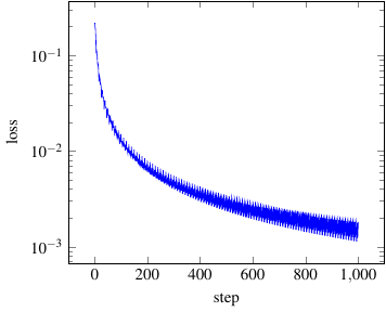
As we see the loss has decreased quite quickly down to 1e-3. Go and have a look at the other columns such as accuracy. Or try to visualize the change in the parameters (weights and biases) in the trajectories dataframe. See 10 Minutes to pandas if we are unfamiliar with the pandas module, yet.
Obviously, we did not use a different dataset set for testing the effectiveness of the training which should commonly be done. This way we cannot check whether we have overfitted or not. However, our example is trivial by design and the network too small to be prone to overfitting this dataset.
Nonetheless, we show how to supply a different dataset and evaluate loss and accuracy on it.
Provide our own dataset
We can directly supply our own dataset, e.g., from a numpy array residing in memory. See the following example where we do not generate the data but parse them from a CSV file instead of using the pandas module.
import TATi.simulation as tati

import numpy as np
import pandas as pd

nn = tati(
    output_activation="linear",
)
# e.g. parse dataset from CSV file into pandas frame
input_dimension = 2
output_dimension = 1
parsed_csv = pd.read_csv("dataset-twoclusters-test.csv", \
                         sep=',', header=0)
# extract feature and label columns as numpy arrays
features = np.asarray(\
    parsed_csv.iloc[:, 0:input_dimension])
labels = np.asarray(\
    parsed_csv.iloc[:, \
        input_dimension:input_dimension \
                        + output_dimension])

# supply dataset (this creates the input layer)
nn.dataset = [features, labels]

# this has created the network, now set
# parameters obtained from optimization run
nn.parameters = np.array([2.42835492e-01, 2.40057245e-01, \
    2.66429665e-03])

# evaluate loss and accuracy
print("Loss: "+str(nn.loss()))
print("Accuracy: "+str(nn.score()))
The major difference is that batch_data_files in tati() is now empty and instead we simply later assign nn.dataset a numpy array to use. Note that we could also have supplied it directly with the filename dataset-twoclusters.csv, i.e. nn.dataset = "dataset-twoclusters.csv". In this example we have parsed the same file as the in the previous section into a numpy array using the pandas module. Natually, this is just one way of creating a suitable numpy array.
At the end we have stated loss() and the score(). While the loss is simply the output of the training function, the score gives the accuracy in a classification problem setting: We compare the label given in the dataset with the label predicted by the network and take the average over the whole dataset (or its mini-batch if batch_size is used). For multi-labels, we use the largest entry as the label in multi classification.
|
Note
|
Input and output dimensions are directly deduced from the the tuple sizes. |
|
Note
|
The nodes in the input layer can be modified using input_columns, e.g., input_columns=["x1", "sin(x2)", "x1^2"]. |
2.2.6. Sampling the network
Typically, as preparation to a sampling run, one would optimize or equilibrate the initially random positions first. This might be considered a specific way of initializing parameters.
|
Note
|
Statistical background
In general, when sampling from a distribution (to compute empirical averages for example), one wants to start close to equilibrium, i.e. from states which are of high probability with respect to the target distribution (therefore the minima of the loss). The initial optimization procedure is therefore a first guess to find such states, or at least to get close to them. |
However, let us first ignore this good practice for a moment and simply look at sampling from a random initial place on the loss manifold. We will come back to it later on.
import TATi.simulation as tati

import numpy as np

nn = tati(
    batch_data_files=["dataset-twoclusters.csv"],
    batch_size=500,
    max_steps=1000,
    output_activation="linear",
    sampler="GeometricLangevinAlgorithm_2ndOrder",
    seed=426,
    step_width=1e-2
)
sampling_data = nn.sample()

print("Sample results")
print(np.asarray(sampling_data.run_info[0:10]))
print(np.asarray(sampling_data.trajectory[0:10]))
print(np.asarray(sampling_data.averages[0:10]))
Here, the sampler setting takes the place of the optimizer before as it states which sampling scheme to use. See [reference.samplers] for a complete list and their parameter names. Apart from that the example code is very much the same as in the example involving fit().
|
Note
|
In the context of sampling we use step_width in place of learning_rate. |
Again, we produce a single data structure that contains three data frames: run info, trajectory, and averages. Trajectories contains among others all parameter degrees of freedom $w=\{w_1, \ldots, w_M\}$ for each step (or every_nth step). Run info contains loss, accuracy, norm of gradient, norm of noise and others, again for each step. Finally, in averages we compute running averages over the trajectory such as average (ensemble) loss, averag kinetic energy, average virial, see general concepts.
Take a peep at sampling_data.run_info.columns to see all columns in the run info dataframe (and similarly for the others.)
For the running averages it is advisable to skip some initial ateps (burn_in_steps) to allow for some burn in time, i.e. for kinetic energies to adjust from initially zero momenta.
Some columns in averages and in run info depend on whether the sampler provides the specific quantity, e.g. SGLD does not have momentum, hence there will be no average kinetic energy.
Using a prior
We may add a prior to the sampling. At the current state two kinds of priors are available: wall-repelling and tethering.
The options prior_upper_boundary and prior_lower_boundary give the admitted interval per parameter. Within a relative distance of 0.01 (with respect to length of domain and only in that small region next to the specified boundary) an additional force acts upon the particles to drives them back into the desired domain. Its magnitude increases with distance to the covered inside the boundary region. The distance is taken to the poour of prior_power. The force is scaled by prior_factor.
In detail, the prior consists of an extra force added to the time integration within each sampler. We compute its magnitude as
where w is the position of the particle, a is the prior_factor, $\pi$ is the position of the boundary (prior_upper_boundary $\pi_{ub}$ or prior_lower_boundary $\pi_{lb}$), and n is the prior_power. Finally, the force is only in effect within a distance of $\tau = 0.01 \cdot || \pi_{ub} - \pi_{lb} ||$ to either boundary by virtue of the Heaviside function $\Theta()$. Note that the direction of the force is such that it always points back into the desired domain.
If upper and lower boundary coincide, then we have the case of tethering, where all parameters are pulled inward to the same point.
At the moment applying prior on just a subset of particles is not supported.
|
Note
|
The prior force is acting directly on the variables. It does not modify momentum. Moreover, it is a force! In other words, it depends on step width. If the step width is too large and if the repelling force increases too steeply close to the walls with respect to the normal dynamics of the system, it may blow up. On the other hand, if it is too weak, then particles may even escape. |
First optimize, then sample
As we have already alluded to before, optimizing before sampling is the recommended procedure. In the following example, we concatenate the two. To this end, we might need to modify some of the options in between. Let us have a look, however with a slight twist.
The dataset shown in Figure Dataset can be even learned by a simpler network: only one of the input nodes is actually needed because of the symmetry.
Hence, we look at such a network by using input_columns to only use input column "x1" although the dataset contains both "x1" and "x2".
Moreover, we will add a hidden layer with a single node and thus obtain a network as depicted in Figure Network. We add this hidden node to make the loss manifold a little bit more interesting.
Additionally, we fix the biases to 0 for both the hidden layer bias and the output bias. Effectively, we have two degrees of freedom left. This is not strictly necessary but allows to plot all degrees of freedom at once.
Finally, we add a prior.
import TATi.simulation as tati

import numpy as np

nn = tati(
    batch_data_files=["dataset-twoclusters.csv"],
    batch_size=500,
    every_nth=100,
    fix_parameters="layer1/biases/Variable:0=0.;output/biases/Variable:0=0.",
    hidden_dimension=[1],
    input_columns=["x1"],
    learning_rate=1e-2,
    max_steps=100,
    optimizer="GradientDescent",
    output_activation="linear",
    sampler = "BAOAB",
    prior_factor=2.,
    prior_lower_boundary=-2.,
    prior_power=2.,
    prior_upper_boundary=2.,
    seed=428,
    step_width=1e-2,
    trajectory_file="trajectory.csv",
)
training_data = nn.fit()

nn.set_options(
    friction_constant = 10.,
    inverse_temperature = .2,
    max_steps = 5000,
)

sampling_data = nn.sample()

print("Sample results")
print(sampling_data.run_info[0:10])
print(sampling_data.trajectory[0:10])
|
Note
|
Setting every_nth large enough is essential when playing around with small networks and datsets as otherwise time spent writing files and adding values to arrays will dominate the actual neural network computations by far. |
As we see, some more options have popped up in the __init__() of the simulation interface: fix_parameters is explained in section [quickstart.simulation.setup.freezing_parameters], hidden_dimension which is a list of the number of hidden nodes per layer, input_columns which contains a list of strings, each giving the name of an input dimension (indexing starts at 1), and all sorts of prior_… that define a wall-repelling prior, again see for details. This will keep parameter values within the interval of [-2,2]. Last but not least, trajectory_file writes all parameters per every_nth step to this file.
Then, we call nn.fit() to perform the training as before.
Next, we need to change the number of steps, set a sampling step width and add the sampler (which might depend on additional parameters, see [reference.samplers] ). This is done by calling nn.set_options().
Having set the stage for the sampling, we commence it by nn.sample().
At the very end we again obtain the data structure containing the pandas DataFrame containing runtime information, trajectory, and averages as its member variables.
|
Warning
|
This time we need the trajectory file for the upcoming analysis. Hence, we write it to a file using the trajectory_file option. Keep the file around as it is needed in the following. |
Let us take a look at the two degrees of freedom of the network, namely the two weights, where we plot one against the other similarly to the Sampled weights before.
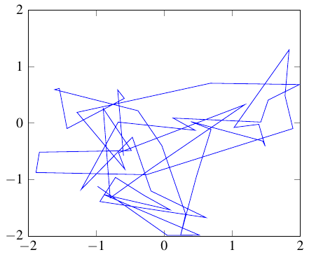
First of all, take note that the prior (given prior_force is strong enough with respect to the chosen inverse_temperature) indeed retains both parameters within the interval [-2,2] as requested.
Compare this to the Figure Loss manifold. we will notice that this trajectory (due to the large enough temperature) has also jumped over the ridge around the origin.
|
Note
|
To bound the runtime of this example, we have set the parameters such that we obtain a good example of a barrier-jumping trajectory. The original values from the introduction are obtained when we reduce the inverse_temperature to 4. and increase max_steps to 20000 (or even more) if we do not mind waiting a minute or two for the sampling to execute. |
2.2.7. Analysing trajectories
Analysis involves parsing in run and trajectory files that we have written during optimization and sampling runs. Naturally, we could also perform this on the pandas dataframes directly, i.e. sampling and analysis in the same python script. However, for completeness we will read from files in the examples of this section.
The analysis functionality has been split into specific operations such as computing averages, computing the covariance matrix or generating a diffusion map analysis. See the source folder src/TAT/analysis, for all contained modules therein each represent such an operation.
In the following we will highlight just a few of them.
All these analysis operations are also possible through TATiAnalyser, see tools/TATiAnalyser.in in the repository.
Average parameters
from TATi.analysis.parsedtrajectory import ParsedTrajectory
from TATi.analysis.averagetrajectorywriter import AverageTrajectoryWriter

trajectory = ParsedTrajectory("trajectory.csv")
avg = AverageTrajectoryWriter(trajectory)
steps = trajectory.get_steps()

print(avg.average_params)
print(avg.variance_params)
We use the helper class ParsedTrajectory which takes a trajectory file and heeds additional options such as neglecting burn in steps or taking only every_nth step into account. Next, we instantiate the AverageTrajectoryWriter module. It computes the averages and variance of each parameter, whose result we print.
AverageTrajectoryWriter can also write the values to a file. Then, two rows are written (together with a header line) in CSV format. The first row (step 0) represents the averages while the second row (step 1) represents the variance of each parameter.
The loss column is the average over all loss values. If an inverse_temperature has been given, then it is the ensemble average, i.e. each loss (and parameter set) is weighted not equivalently but by $exp(-\beta L)$.
In general, taking such an average is only useful if the trajectory has remained essentially within a single minimum. If the loss manifold has the overall shape of a large funnel with lots of local minima at the bottom, this may be feasible as well.
|
Note
|
Averages depend crucially on the number of steps we average over. I.e. the more points we throw away (option every_nth), the less accurate it becomes. In other words, if large accuracy is required, the averages data frame (if it contains the value of interest) is a better place to look for. |
Covariance
The covariance matrix of the trajectory gives the joint variability of any two of its components. Its eigenvalues give a notion the magnitude between directions with large gradients and between directions with small gradients.
In sampling this is important as directions with small gradients take longer to be explored, see the concept of Integrated Autocorrelation Time (IAT) in section [quickstart.sampling.iat].
|
Note
|
If we look at the covariance of a distribution, we essentially replace it by a Gaussian mixture model defined by this covariance matrix. |
Let us compute the covariance using the analysis module Covariance.
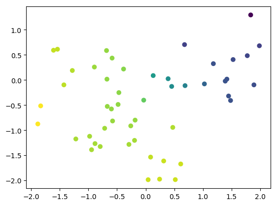
import numpy as np
import matplotlib

# use agg as backend to allow command-line use as well
matplotlib.use("agg")
import matplotlib.pyplot as plt

from TATi.analysis.parsedtrajectory import ParsedTrajectory
from TATi.analysis.covariance import Covariance

trajectory = ParsedTrajectory("trajectory.csv")

num_eigenvalues=2
cov = Covariance(trajectory)
cov.compute( \
    number_eigenvalues=num_eigenvalues)

# plot in eigenvector directions
x = np.matmul(trajectory.get_trajectory(), cov.vectors[:,0])
y = np.matmul(trajectory.get_trajectory(), cov.vectors[:,1])
plt.scatter(x,y, marker='o', c=-x)
plt.savefig('covariance.png', bbox_inches='tight')
#plt.show()
Note the helper class ParsedTrajectory which takes a trajectory file and heeds additional options such as neglecting burn in steps or taking only every_nth step into account. This instance is handed to the Covariance class whose compute() function performs the actual analysis. Typicallay, all analysis operations have such a compute() function. Again, we plot the result.
We have depicted the weights in the direction of each eigenvector. Essentially, we get a rotated view of the trajectory in [quickstart.simulation.analysis.optimize_sample.weights] where the x direction represents the dominant change.
Diffusion Map
Diffusion maps are a technique for unsupervised learning introduced by [Coifman2006].
Diffusion maps is a dimension reduction technique that can be used to discover low dimensional structure in high dimensional data. It assumes that the data points, which are given as points in a high dimensional metric space, actually live on a lower dimensional structure. To uncover this structure, diffusion maps builds a neighborhood graph on the data based on the distances between nearby points. Then a graph Laplacian L is constructed on the neighborhood graph. Many variants exist that approximate different differential operators.
— pydiffmap
pydiffmap is an excellent Python package that performs the analysis which consists of computing the eigendecomposition of a sparse neighborhood graph where the Euclidean metric is used as distance measure. If it is installed (using pip), it is used for this type of analysis (use method=pydiffmap in this case).
In a nutshell, the eigenvectors of the diffusion map kernel give us the main directions on our trajectory. They represent collective variables learned from the trajectory.
Let us take a look at the eigenvectors from our trajectory that we have sampled just before.
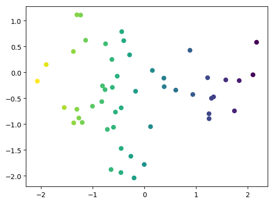
import matplotlib

# use agg as backend to allow command-line use as well
matplotlib.use("agg")
import matplotlib.pyplot as plt

from TATi.analysis.parsedtrajectory import ParsedTrajectory
from TATi.analysis.diffusionmap import DiffusionMap

# option values coming from the sampling
inverse_temperature=2e-1

trajectory = ParsedTrajectory("trajectory.csv")

num_eigenvalues=2
dmap = DiffusionMap.from_parsedtrajectory(trajectory)
dmap.compute( \
    number_eigenvalues=num_eigenvalues,
    inverse_temperature=inverse_temperature,
    diffusion_map_method="vanilla",
    use_reweighting=False)

plt.scatter(trajectory.get_trajectory()[:,0], trajectory.get_trajectory()[:,1], c=dmap.vectors[:,0])
plt.savefig('eigenvectors.png', bbox_inches='tight')
#plt.show()
We should then obtain the Figure Diffusion map analysis.
|
Note
|
The true first eigenvector is constant and is therefore dropped in the function compute_diffusion_maps(). |
Keep in mind that the ridge is at the origin and there are two hperbolic basins on either side in the all-positive and all-negative orthant of the 2d space. We see that as we color the trajectory points by the value of the dominant eigenvector, the path between these two minima is highlighted: from light green to dark blue.
The eigenvector gives a direction: From the top right to the bottom left and therefore from one minimum basin to the other.
The eigenvector component give the implicit evaluation of the collective variable function at each trajectory point, i.e. $e_i = \xi(x_i)$, where $\xi(x)$ is the collective variable and $e_i$ is the i-th component and $x_i$ the i-th trajectory point.
The eigenvectors of the diffusion map kernel also give us a mean to assess distances between trajectory points by looking at the difference in values, $|e_i - e_j|$. This is the so-called diffusion distance. It tells us how difficult it is to diffuse from one point to the other.
The main difference between the covariance and diffusion maps is that the latter gives a non-linear mapping which is much more powerful.
2.2.8. Conclusion
This has been the quickstart introduction to the simulation interface.
If we want to take this further, we recommend reading how to implement a GLA2 sampler using this module.
If we still want to take it further, then we need to look at the programmer’s guide that should accompany our installation.
2.3. Using command-line interface
All the tests use the command-line interface which suits itself well for performing rigorous scientific experiments in scripted stages. We recommend using this interface when doing parameter studies and performing extensive runs using different seeds.
The examples on this interface will be much briefer as you are hopefully aware of the simulation module quickstart already and therefore much should be familiar.
|
Note
|
All command-line option have equivalently named counterparts in the options given to the simulation (or model) module on instantiation or to simulation.set_options(), respectively. |
2.3.1. Creating the dataset
As data is read from file, this file needs to be created beforehand.
For a certain set of simple classification problems, namely those that can be found in the tensorflow playground, we have added a TATiDatasetWriter that spills out the dataset in CSV format.
TATiDatasetWriter \
        --data_type 2 \
        --dimension 500 \
        --noise 0.1 \
        --seed 426 \
        --train_test_ratio 0 \
        --test_data_file testset-twoclusters.csv
This will write 500 datums of the dataset type 2 (two clusters) to a file testset-twoclusters.csv using all of the points as we have set the test/train ratio to 0. Note that we also perturb the points by 0.1 relative noise.
2.3.2. Parsing the dataset
Similarly, for testing the dataset can be parsed using the same tensorflow machinery as is done for sampling and optimizing, using
TATiDatasetParser \
    --batch_data_files dataset-twoclusters.csv \
    --batch_size 20 \
    --seed 426
where the seed is used for shuffling the dataset.
This will print 20 randomly drawn items from the dataset.
2.3.3. Optimizing the network
As weights (and biases) are usually uniformly random initialized and the potential may therefore start with large values, we first have to optimize the network, using (Stochastic) Gradient Descent (GD).
2.3.4. Freezing parameters
Sometimes it might be desirable to freeze parameters during training or sampling. This can be done as follows:
from TATi.model import Model as tati

import numpy as np

FLAGS = tati.setup_parameters(
    batch_data_files=["dataset-twoclusters-small.csv"],
    fix_parameters="output/biases/Variable:0=2.",
    max_steps=5,
    seed=426,
)

nn = tati(FLAGS)
nn.init_input_pipeline()
nn.init_network(None, setup="train")
nn.reset_dataset()
run_info, trajectory, _ = nn.train(return_run_info=True, \
  return_trajectories=True)

print("Train results")
print(np.asarray(trajectory[0:5]))
Note that we fix the parameter where we give its name in full tensorflow namescope: "layer1" for the network layer, "weights" for the weights ("biases" alternatively) and "Variable:0" is fixed (as it is the only one). This is followed by a comma-separated list of values, one for each component.
|
Note
|
Single values cannot be frozen but only entire weight matrices or bias vectors per layer at the moment. As each component has to be listed, at the moment this is not suitable for large vectors. |
TATiOptimizer \
    --batch_data_files dataset-twoclusters.csv \
    --batch_size 50 \
    --loss mean_squared \
    --learning_rate 1e-2 \
    --max_steps 1000 \
    --optimizer GradientDescent \
    --run_file run.csv \
    --save_model `pwd`/model.ckpt.meta \
    --seed 426 \
    -v
This call will parse the dataset from the file dataset-twoclusters.csv. It will then perform a (Stochastic) Gradient Descent optimization in batches of 50 (10% of the dataset) of the parameters of the network using a step width/learning rate of 0.01 and do this for 1000 steps after which it stops and writes the resulting neural network in a TensorFlow-specific format to a set of files, one of which is called model.ckpt.meta (and the other filenames are derived from this).
We have also created a file run.csv which contains among others the loss at each (every_nth, respectively) step of the optimization run. Plotting the loss over the step column from the run file will result in a figure similar to in Loss history.
|
Note
|
Since Tensorflow 1.4 an absolute path is required for the storing the model. In the example we use the current directory returned by the unix command pwd. |
If you need to compute the optimal step width, which is possible for smaller networks from the largest eigenvalue of the hessian matrix, then use the option do_hessians 1 to activate it.
|
Note
|
The creation of the nodes is costly, $O(N^2)$ in the number of parameters of the network N. Hence, may not work for anything but small networks and should be done on purpose. |
2.3.5. Sampling trajectories on the loss manifold
Next, we show how to use the sampling tool called TATiSampler.
TATiSampler \
    --averages_file averages.csv \
    --batch_data_files dataset-twoclusters.csv \
    --batch_size 50 \
    --friction_constant 10 \
    --inverse_temperature 10 \
    --loss mean_squared \
    --max_steps 1000 \
    --sampler GeometricLangevinAlgorithm_2ndOrder \
    --run_file run.csv \
    --seed 426 \
    --step_width 1e-2 \
    --trajectory_file trajectory.csv
This will cause the sampler to parse the same dataset as before. Afterwards it will use the GeometricLangevinAlgorithm_2nd order discetization using again step_width of 0.01 and running for 1000 steps in total. The GLA is a descretized variant of Langevin Dynamics whose accuracy scales with the inverse square of the step_width (hence, 2nd order).
The seed is needed as we sample using Langevin Dynamics where a noise term is present whose magnitude scales with inverse_temperature.
After it has finished, it will create three files; a run file run.csv containing run time information such as the step, the potential, kinetic and total energy at each step, a trajectory file trajectory.csv with each parameter of the neural network at each step, and an averages file averages.csv containing averages accumulated along the trajectory such as average kinetic energy, average virial ( connected to the kinetic energy through the virial theorem, valid if a prior keeps parameters bound to finite values), and the average (ensemble) loss. Moreover, for the HMC sampler the average rejection rate is stored there. The first two files we need in the next stage.
As it is good practice to first optimize and then sample, also referred as to start from an equilibrated position, we may load the model saved after optimization by adding the option:
...
  --restore_model ‘pwd‘/model.ckpt.meta \
...
Otherwise we start from randomly initialized weights and non-zero biases.
2.3.6. Analysing trajectories
Eventually, we now want to analyse the obtained trajectories. The trajectory file written in the last step is simply a matrix of dimension (number of parameters) times (number of trajectory steps).
The analysis can perform a number of different operations where we name a few:
-
Calculating averages.
-
Calculating covariances.
-
Calculating the diffusion map’s largest eigenvalues and eigenvectors.
-
Calculating landmarks and level sets to obtain an approximation to the free energy.
Averages
Averages are calculated by specifying two options as follows:
TATiAnalyser \
    average_energies average_trajectory \
    --average_run_file average_run.csv \
    --average_trajectory_file average_trajectory.csv \
    --drop_burnin 100 \
    --every_nth 10 \
    --run_file run.csv \
    --steps 10 \
    --trajectory_file trajectory.csv
This will load both the run file run.csv and the trajectory file trajectory.csv` and average over them using only every 10 th data point (every_nth) and also dropping the first steps below 100 (drop_burnin). It will produce then ten averages (steps) for each of energies in the run file and each of the parameters in the trajectories file (along with the variance) from the first non-dropped step till one of the ten end steps. These end steps are obtained by equidistantly splitting up the whole step interval.
Eventually, we have two output file. The averages over the run information such as total, kinetic, and potential energy in average_run.csv. Also, we have the averages over the degrees of freedom in average_trajectories.csv.
This second file contains two rows (together with a header line) in CSV format. The first row (step 0) represents the averages while the second row (step 1) represents th variance of each parameter.
The loss column is the average over all loss values. If an inverse_temperature has been given, then it is the ensemble average, i.e. each loss (and parameter set) is weighted not equivalently (unit weight) but by $exp(-\beta L)$.
In general, taking such an average is only useful if the trajectory has remained essentially within a single minimum. If the loss manifold has the overall shape of a large funnel with lots of local minima at the bottom, this may be feasible as well. Use a covariance analysis and TATiLossFunctionSampler in directions of eigenvalues of the resulting covariance matrix whose magnitude is large to find out.
|
Note
|
Averages depend crucially on the number of steps we average over. I.e. the more points we throw away (option every_nth), the less accurate it becomes. In other words, if large accuracy is required, the averages file (if it contains the value of interest) is a better place to look for. |
Covariance
Computing the covariance is done as follows.
TATiAnalyser \
    covariance \
    --covariance_matrix covariance.csv \
    --covariance_eigenvalues eigenvalues.csv \
    --covariance_eigenvectors eigenvectors.csv \
    --drop_burnin 100 \
    --every_nth 10 \
    --number_of_eigenvalues 3 \
    --trajectory_file trajectory.csv
Here, we simply give the respective options to write the covariance matrix, its eigenvectors and eigenvalues to CSV files. We drop the first 100 steps and take only every 10th step into account.
The covariance eigenvectors give use the directions of strong and weak change while the eigenvalues give their magnitude. This correlates with strong and weak gradients and therefore with general directions of fast and slow exploration.
Diffusion map
See section [quickstart.simulation.analysis.diffusion_map] for some more information on diffusion maps.
its eigenvalues and eigenvectors can be written as well to two output files.
TATiAnalyser \
    diffusion_map \
    --diffusion_map_file diffusion_map_values.csv \
    --diffusion_map_method vanilla \
    --diffusion_matrix_file diffusion_map_vectors.csv \
    --drop_burnin 100 \
    --every_nth 10 \
    --inverse_temperatur 1e4 \
    --number_of_eigenvalues 4 \
    --steps 10 \
    --trajectory_file trajectory.csv
The files ending in ..values.csv contains the eigenvalues in two columns, the first is the eigenvalue index, the second is the eigenvalue.
The other file ending in ..vectors.csv is simply a matrix of the eigenvector components in one direction and the trajectory steps in the other. Additionally, it contains the parameters at the steps and also the loss and the kernel matrix entry.
Note that again the all values up till step 100 are dropped (due to option drop_burnin) and only every 10th trajectory point (due to option every_nth) is considered afterwards.
There are two methods available. Here, we have used the simpler (and less accurate) (plain old) vanilla method. The other is called TMDMap.
If you have installed the pydiffmap python package, this may also be specified as diffusion map method. It has the benefit of an internal optimal parameter choice. Hence, it should behave more robustly than the other two methods. TMDMap is different only in re-weighting the samples according to the specific temperature.
2.3.7. More tools
There are a few more tools available in TATi. They allow to inspect the loss manifold or the input space with respect to a certain parameter set.
The loss function
Let us give an example call of TATiLossFunctionSampler right away.
TATiLossFunctionSampler \
  trajectory \
  --batch_data_files dataset-twoclusters.csv \
  --batch_size 20 \
  --csv_file TATiLossFunctionSampler-output-SGLD.csv \
  --parse_parameters_file trajectory.csv
It takes as input the dataset file dataset-twoclusters.csv and either a parameter file trajectory.csv. This will cause the program the re-evaluate the loss function at the trajectory points which should hopefully give the same values as already stored in the trajectory file itself.
However, this may be used with a different dataset file, e.g. the testing or validation dataset, in order to evaluate the generalization error in terms of the overall accuracy or the loss at the points along the given trajectory.
Interesting is also the second case, where instead of giving a parameters file, we sample the parameter space equidistantly as follows:
TATiLossFunctionSampler \
  naive_grid \
  --batch_data_files dataset-twoclusters.csv \
  --batch_size 20 \
  --csv_file TATiLossFunctionSampler-output-SGLD.csv \
  --interval_weights -5 5 \
  --interval_biases -1 1 \
  --samples_weights 10 \
  --samples_biases 4
Here, sample for each weight in the interval [-5,5] at 11 points (10
endpoint), and similarly for the weights in the interval [-1,1] at 5
points.
|
Note
|
For anything but trivial networks the computational cost quickly becomes prohibitively large. However, we may use fix_parameter to lower the computational cost by choosing a certain subsets of weights and biases to sample. |
TATiLossFunctionSampler \
  naive_grid \
  --batch_data_files dataset-twoclusters.csv \
  --batch_size 20 \
  --csv_file TATiLossFunctionSampler-output-SGLD.csv \
  --fix_parameters "output/weights/Variable:0=2.,2." \
  --interval_weights -5 5 \
  --interval_biases -1 1 \
  --samples_weights 10 \
  --samples_biases 4
Moreover, using exclude_parameters can be used to exclude parameters from the variation, i.e. this subset is kept at fixed values read from the file given by parse_parameters_file where the row designated by the value in parse_steps is taken.
This can be used to assess the shape of the loss manifold around a found minimum.
TATiLossFunctionSampler \
  naive_grid \
  --batch_data_files dataset-twoclusters.csv \
  --batch_size 20 \
  --csv_file TATiLossFunctionSampler-output-SGLD.csv \
  --exclude_parameters "w1" \
  --interval_weights -5 5 \
  --interval_biases -1 1 \
  --parse_parameters_file centers.csv \
  --parse_steps 1 \
  --samples_weights 10 \
  --samples_biases 4 \
  -vv
Here, we have excluded the second weight, named w1, from the sampling. Note that all weight and all bias degrees of freedom are simply enumerated one after the other when going from the input layer till the output layer.
Furthermore, we have specified a file containing center points for all excluded parameters. This file is of CSV style having a column step to identify which row is to be used and moreover a column for every (excluded) parameter that is fixed at a value unequal to 0. Note that the minima file written by TATiExplorer can be used as this centers file. Moreover, also the trajectory files have the same structure.
The learned function
The second little utility programs does not evaluate the loss function itself but the unknown function learned by the neural network depending on the loss function, called the TATiInputSpaceSampler. In other words, it gives the classification result for data point sampled from an equidistant grid. Let us give an example call right away.
TATiInputSpaceSampler \
        --batch_data_files grid.csv \
        --csv_file TATiInputSpaceSampler-output.csv \
        --input_dimension 2 \
        --interval_input -4 4 \
        --parse_steps 1 \
        --parse_parameters_file trajectory.csv \
        --samples_input 10 \
        --seed 426
Here, batch_data_files is an input file but it does not need to be present. (Sorry about that abuse of the parameter as usually batch_data_files is read-only. Here, it is overwritten!). Namely, it is generated by the utility in that it equidistantly samples the input space, using the interval [-4,4] for each input dimension and 10+1 samples (points on -4 and 4 included). The parameters file trajectory.csv now contains the values of the parameters (weights and biases) to use on which the learned function depends or by, in other words, by which it is parametrized. As the trajectory contains a whole flock of these, the parse_steps parameter tells it which steps to use for evaluating each point on the equidistant input space grid, simply referring to rows in said file.
|
Note
|
For anything but trivial input spaces the computational cost quickly becomes prohibitively large. But again fix_parameters is heeded and can be used to fix certain parameters. This is even necessary if parsing a trajectory that was created using some parameters fixed as they then will not appear in the set of parameters written to file. This will raise an error as the file will contain too few values. |
2.4. Conclusion
This has been the quickstart introduction.
In the following reference section you may find the following pieces interesting after having gone through this quickstart tutorial.
-
[reference.examples.harmonic_oscillator] for a light-weight example probability distribution function whose properties are well understood.
-
[reference.implementing_sampler] explaining how to implement your own sampler using the Simulation module as rapid-prototyping framework.
-
[reference.simulation] giving detailed examples on each function in Simulationss interface.
3. The reference
3.1. General concepts
Here, we give definitions on a number of concepts that occur throughout this userguide.
-
Dataset
The dataset $D = \{X,Y\}$ contains a fixed number of datums of input tuples or features $X=\{x_d\}$ and output tuples or labels $Y=\{y_d\}$. Basically, they are samples taken from the unknown function which we wish to approximate using the neural network. If the output tuples are binary in each component, the approximation problem is called a classification problem. Otherwise, it is a regression problem.
-
Neural network
The neural network is a black-box representing a certain set of general functions that are efficient in solving classification problems (among others). They are parametrized explicitly using weights and biases $w=\{w_1, \ldots, w_M\}$ and implicitly through the topology of the network (connections of nodes residing in layers) and the activation functions used. The network’s output $F_w(x_i)$ depends explicitly on the dataset’s current datum (fed into the network) and implicitly on the parameters.
-
Loss
The default is mean_squared.
The loss function $L_D(w)$ determines for a given (labeled) dataset what set of neural network’s parameters are best. Different losses result in different set of parameters. It is a high-dimensional manifold that we want to learn and capture using the neural network. It implicitly depends on the given dataset and explicitly on the parameters of the neural network, namely weights and biases, $w=\{w_1, \ldots, w_M\}$.
Most important to understand about the loss is that it is a non-convex function and therefore in general does not just have a single minimum. This makes the task of finding a good set of parameters that (globally) minimize the loss difficult as one would have to find each and every minima in this high-dimensional manifold and check whether it is actually the global one.
-
Momenta and kinetic energy
Momenta $p=\{p_1, \ldots, p_M\}$ is a concept taken over from physics where the parameters are considered as particles each in a one-dimensional space where the loss is a potential function whose ( negative) gradient acts as a force onto the particle driving them down-hill (towards the local minimum). This force is integrated in a classical Newton’s mechanic style, i.e. Newton’s equation of motion is discretized with small time steps (similar to the learning rate in Gradient Descent). This gives first rise to/velocity and second to momenta, i.e. second order ordinary differential equation (ODE) split up into a system of two one-dimensional ODEs. There are numerous stable time integrators, i.e. velocity Verlet/Leapfrog, that are employed to propagate both particle position (i.e. the parameter value) and its momentum through time. Note that momentum and velocity are actually equivalent as usually the mass is set to unity.
The kinetic energy $0.5 \sum^M_i p^T_i p_i$ is computed as sum over kinetic energies of each parameter.
-
Virial
Virial $0.5 \sum^M_i w^T_i \nabla_{w_i} L_D(w)$ is defined as one half of the sum over the scalar product of gradients with parameters. Given that the loss function is unbounded from above and raises more quickly than a linear function, the asymptotic value of the virial is related to the average kinetic energy through the virial theorem, see https://en.wikipedia.org/wiki/Virial_theorem.
-
Averages
Averages are meaningful when looking at the probability distribution function instead of the loss directly, see Section [quickstart.sampling.sequences]. There, we compute the integral $\int A(w,p) \mu(w,p)$ for in our case the (canonical) Gibbs measure $\mu(w,p) = \exp(-\beta L_D(w))$ that turns the loss into probability distribution function. Here, $A(w,p)$ is an observable, i.e. a function depending on positions and momenta. Examples of such observables are the kinetic energy or the virial, or maybe the parameters themselves.
3.2. Examples
We show how to set up some basic models, which can be a useful tool to study and test methods.
3.2.1. Harmonic oscillator
It can be sometimes useful to use TATi to simulate a simple harmonic oscillator. This model can be obtained by training the neural network with one parameter on one point $X=1$ in dimension one with a label equal to zero, i.e. $Y=0$, and using the mean square loss function and linear activation function. More precisely, the cost function becomes in this setting:
$L(\omega | X,Y) = | \omega X + b - Y|^2$,
where we fix the bias $b=0$.
-
Dataset:
from TATi.common import data_numpy_to_csv
import numpy as np

X = np.asarray([[1]])
Y = np.asarray([[0]])

# prepare and save the trivial data set for later
datasetName = 'dataset_ho.csv'
data_numpy_to_csv(X, Y, datasetName)
numberOfPoints = 1
-
Setup and train neural network:
import TATi.simulation as tati import numpy as np import pandas as pd nn = tati( batch_data_files=["dataset_ho.csv"], batch_size=1, fix_parameters="output/biases/Variable:0=0.", friction_constant=10.0, input_dimension=1, inverse_temperature=1.0, loss="mean_squared", max_steps=1000, output_activation = "linear", output_dimension=1, run_file="run_ho.csv", sampler="BAOAB", seed=426, step_width=0.5, trajectory_file="trajectory_ho.csv", verbose=1 ) data = nn.sample() df_trajectories = pd.DataFrame(data.trajectory) # sampled trajectory weight0 = np.asarray(df_trajectories['weight0']) -
Sampled trajectory:
The output trajectory in trajectory_ho.csv or weight0 is distributed w.r.t. a Gaussian, i.e. the density of X:=weight0 is $exp(-X^2)$, see Figure Gaussian distribution.
|
Note
|
The figure was obtained with setting max_steps to 10000. |
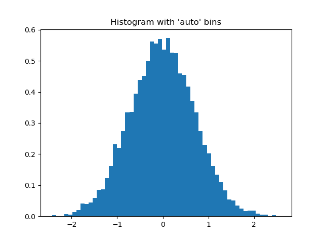
3.3. Optimizers
Optimizers in TATi primarily serve the purpose of finding a good starting position for the samplers.
To this end, only a few optimizers are currently implemented.
-
(Stochastic) Gradient Descent
-
Gradient Descent with step width calculated following Barzilai-Borwein
3.3.1. Gradient Descent
optimizer: GradientDescent
This implementation directly calls upon Tensorflow’s GradientDescentOptimizer. It is slightly modified for additional book-keeping of norms of gradients and the virial (this can be deactivated setting do_accumulates to False).
The step update is: $\theta^{n+1} = \theta^{n} - \nabla U(\theta) \Delta t$,
3.3.2. Gradient Descent with Barzilai-Borwein step width
optimizer: BarzilaiBorweinGradientDescent
The update step is the same as for [reference.optimizers.gd]. However, the learning rate $\Delta t$ is modified as, see [Barzilai1988],
$\Delta t = \frac{ (\theta^{n} - \theta^{n-1})\cdot(\nabla U(\theta^{n})- \nabla U(\theta^{n-1})) }{ |(\nabla U(\theta^{n})- \nabla U(\theta^{n-1})|^2 }$.
where the learning rate is bounded in the interval [1e-10,1e+10] to ensure numerical stability. If the above calculation should be invalid, the default learning rate $\Delta t$ is used.
3.4. Samplers
Samplers are discretizations of a given dynamical system, set by an ODE or SDE. In our case, it is mostly Langevin dynamics. Given that the sampler is ergodic we can replace integrals over the whole domain by integrals along sufficiently long trajectories.
Certain asymptotical properties are inherently connected to the respective dynamics, for example, the average kinetic energy. It can be evaluated as an average by integrating along the trajecories. However, as it is not possible to integrate the continuous dynamics directly, we rely on the respective discretization, the sampler, which naturally introduces an error.
This discretization error depends on the chosen finite step width by which the trajectories are produced. It shows as a finite error to the asymptotical value regardless of the length of the trajectory. Choosing a smaller step width will produce a smaller error.
This can be observed for the average kinetic energy by looking at a small example network and dataset and producing sufficiently long trajectories. If one plots the difference against the known asymptotical value (namely $\frac{N^{dof}}{2} k_B T$ with temperature T, and degrees of freedom $N^{dof}$) over different step widths in double logarithmic fashion, one obtains straight lines whose slope depends on the discretization order.
Different samplers have different discretization orders and the order also depends on the observed quantity.
This makes picking the right sampler a critical choice: From a statistical point of view the most accurate sampler is best, i.e. the one having the highest discretization order. Also, as all of them have roughly the same computational cost, it is generally recommended to pick BAOAB which has second order convergence and even fourth order in the high-friction limit, see [Leimkuhler2012] for details.
|
Note
|
At the beginning of each the following subsections we give the name of the respective sampler in order to activate it using the sampler keyword, see [quickstart.simulation.sampling] and [quickstart.cmdline.sampling]. |
|
Note
|
In explaining implementation details, we will be using the B,A,O notation for giving the order of the split analytic integration steps: B means momentum integration, A stands for position integration and O is associated with the noise step. |
3.4.1. Stochastic Gradient Langevin Dynamics
sampler: StochasticGradientLangevinDynamics
The Stochastic Gradient Langevin Dynamics (SGLD) was proposed by [Welling2011] based on the [SGD][Stochastic Gradient Descent], which is a variant of the [GD][Gradient Descent] using only a subset of the dataset for computing gradients. The central idea behind SGLD was to add an additional noise term whose magnitude then controls the noise induced by the approximate gradients. By a suitable reduction of the step width the method can be shown to be globally convergent. This reduction is typically not done in practice.
Implements a Stochastic Gradient Langevin Dynamics Sampler in the form of a TensorFlow Optimizer, overriding tensorflow.python.training.Optimizer.
The step update is: $\theta^{n+1} = \theta^{n} - \nabla U(\theta) \Delta t + \sqrt{\frac{2\Delta t} {\beta}} G^n$, where $\beta$ is the inverse temperature coefficient, $\Delta t$ is the (discretization) step width and $\theta$ is the parameter vector, $U(\theta)$ the energy or loss function, and $G\sim N (0, 1)$.
| Option name | Description |
|---|---|
step_width |
time integration step width $\delta t$ |
|
Note
|
SGLD is very much like SGD and GD in terms that the step_width needs to be small enough with respect to the gradient sizes of your problem. |
3.4.2. Covariance Controlled Adaptive Langevin
sampler: CovarianceControlledAdaptiveLangevin
This is an extension of Stochastic Gradient Descent proposed by [Shang2015]. The key idea is to dissipate the extra heat caused by the approximate gradients through a suitable thermostat. However, the discretisation used here is not based on the (first-order) Euler-Maruyama as [SGLD] but on [GLA] 2nd order.
| Option name | Description |
|---|---|
friction_constant |
friction constant $\gamma$ that controls how much momentum is replaced by random noise each step |
inverse_temperature |
inverse temperature factor scaling the noise, $\beta$ |
sigma |
controlling the thermostat |
sigmaA |
controlling the thermostat’s adaptivity |
step_width |
time integration step width $\delta t$ |
|
Note
|
sigma and sigmaA are two additional parameters that control the action of the thermostat. Moreover, we require the same parameters as for [GLA] 2nd order. |
3.4.3. Geometric Langevin Algorithms
sampler: Geometric Langevin Algorithms_1stOrder, Geometric Langevin Algorithms_2ndOrder
GLA results from a first-order splitting between the Hamiltonian and the Ornstein-Uhlenbeck parts, see [Leimkuhler2015][section 2.2.3, Leimkuhler 2015] and also [Leimkuhler2012]. If the Hamiltonian part is discretized with a scheme of second order as in GLA2, it provides second order accuracy at basically no extra cost.
The update step of the parameters for second order GLA is BABO:
$B: p^{n+1/2} = p^n -\nabla U(q^n)\frac{\Delta t}{2}$
$A: q^{n+1} =q^n+M^{-1}p^{n+1/2}\Delta t$
$B: \tilde{p}^{n+1} = p^{n+1/2} -\nabla U(q^{n+1})\frac{\Delta t}{2}$
$O: p^{n+1} = \alpha_{\Delta t}\tilde{p}^{n+1}+ \sqrt{\frac{1-\alpha_{\Delta t}^2}{\beta}M}G^n$ where $\alpha_{\Delta t}=exp(-\gamma \Delta t)$ and $G\sim N (0, 1)$.
The first order GLA is BAO.
| Option name | Description |
|---|---|
friction_constant |
friction constant $\gamma$ that controls how much momentum is replaced by random noise each step |
inverse_temperature |
inverse temperature factor scaling the noise, $\beta$ |
step_width |
time integration step width $\delta t$ |
|
Note
|
All GLA samplers have two more parameters: inverse_temperature (usually denoted as $\beta$) and friction_constant (usually denoted as $\gamma$). Inverse temperature controls the average momentum of each parameter while the friction constant decides over how much of the momentum is replaced by random noise, i.e. the random walker character of the trajectory. Good values for beta depend on the loss manifold and its barriers and need to be find by try&error at the moment. As a rough guide, $\gamma=10$ is a good start for the friction constant. Moreover, when choosing such a friction constant, with $\beta=1000$ sampling will remain in the starting minimum basin, while $\beta=1$ exists basins very soon. Note that large noise can be hidden by a too small friction constant, i.e. they both depend on each other. |
Implementation notes
The first order GLA with its BAO sequence of steps is implemented in a straight-forward fashion. GLA2 with its BABO sequence is more difficult as we would need to calculate the updated gradients for the second "B" step. Tensorflow, however, by its code design, only allows gradient (and loss) evaluation at the very beginning of the sequence.
To overcome this, we shuffle the steps in a cyclic fashion to become BOBA. This can be seen as delaying some steps at iteration $n$ and performing them at iteration $n+1$. Here, we delay the action of the "BO" part to the next step.
When doing this, we have to take extra care to still calculate all energies at the correct time: the only "A" step is the last and loss evaluation is at the right moment. Moreover, both "B" steps now use the same gradient and we do not need to recalculate. The only minor difficulty is that the kinetic energy must be evaluated after the "O" step. This is no problem as the kinetic energy is not computed by Tensorflow and therefore we are not constrained.
|
Note
|
This cyclic permutation still changes the very first step that is however typically started from a random position. Hence, this has no effect. |
3.4.4. BAOAB
sampler: BAOAB
BAOAB derives from the basic building blocks A (position update), B (momentum update), and O (noise update) into which the Langevin system is split up. Each step is solved in a separate step. Hence, we perform a B step, then an A step, … and so on. This scheme has second-order accuracy and superb overall accuracy with respect to positions. See [Leimkuhler2012] for more details.
The update step of the parameters is:
$B: p^{n+1/2} = p^n -\nabla U(q^n)\frac{\Delta t}{2}$
$A: q^{n+1} =q^n+M^{-1}p^{n+1/2}\frac{\Delta t}{2}$
$O: p^{n+1} = \alpha_{\Delta t}\tilde{p}^{n+1}+ \sqrt{\frac{1-\alpha_{\Delta t}^2}{\beta}M}G^n$
$A: q^{n+1} =q^n+M^{-1}p^{n+1/2}\frac{\Delta t}{2}$
$B: p^{n+1/2} = p^n -\nabla U(q^n)\frac{\Delta t}{2}$
where $\alpha_{\Delta t}=exp(-\gamma \Delta t)$ and $G\sim N (0, 1)$.
| Option name | Description |
|---|---|
friction_constant |
friction constant $\gamma$ that controls how much momentum is replaced by random noise each step |
inverse_temperature |
inverse temperature factor scaling the noise, $\beta$ |
step_width |
time integration step width $\delta t$ |
Implementation notes
With BAOAB we face similar difficulties as with second order GLA: we would need to recalculate gradients for the second "B" step. Again, we solve this by cyclic permutation of the steps to become BBAOA. In other words, we delay the action of the very last "B" step to iteration $n+1$.
Now, gradient calculation is at the very beginning and both "B" steps use the same gradient. Loss calculation is still after the second "A" step. The only minor difficulty is again calculating the kinetic energy: this needs to occur in between the two "B" steps. Naturally, this is now also delayed to the next step. However, as the loss is always computed prior to updating the state they still match.
3.4.5. Hamiltonian Monte Carlo
sampler: HamiltonianMonteCarlo_1stOrder (modified Euler), HamiltonianMonteCarlo_2ndOrder (Leapfrog)
HMC is based on Hamiltonian dynamics instead of Langevin Dynamics. Noise only enters when, after the evaluation of an acceptance criterion, the momenta are redrawn randomly. It has first been proposed by [Duane1987].
This Metropolisation ensures that too large step widths will not negatively affect the sampled distribution. In contrast to the sampling through Langevin Dynamics there is no bias with respect to the step width. However, a large step width will potentially cause a higher rejection rate.
One further virtue of HMC is when using longer Verlet time integration legs (hamiltonian_dynamics_time larger than step_width) that the walker will progress much further than in the case of Langevin Dynamics. This is because it only uses the gradient. In contrast to samplers based on Langevin dynamics, it is not performing partly a Brownian motion through the injected noise. Langevin dynamics can be recovered by using just a single step for time integration (i.e. a single step is immediately followed by evaluating the acceptance criterion). This is called "Langevin Monte Carlo" which does however lack the favorable scaling properties of HMC, i.e. when using multiple steps. Random walk scales as $d^2$ in the amount of computation time for a dataset of dimensionality $d$, while HMC scales only as $d^{5/4}$. LMC on the other hand scales as $d^{4/3}$, see Neal, 2011, section 4.4 and 5.2.
However, longer legs again typically cause higher rejection rates. Therefore, they come at the price of extra computational work in terms of possibly rejected legs. There are specific rejection rates that are optimal. Typically they range between 35% ($L\gg 1$) and 43% ($L=1$). In essence, the rejection rate tells about getting sufficiently far from the initial state to a truly independent proposal state. See Neal, 2011, section 5.2 for details and in general [Neal2011] for a very readable, general introduction to HMC in the context of Markov Chain Monte Carlo methods.
| Option name | Description |
|---|---|
hamiltonian_dynamics_time |
Time used for integrating Hamiltonian dynamics. This is relative to step_width. For example, if step_width is 0.05 and this is chosen as 0.05 as well, it will evaluate every other step, i.e. perform only a single time integration step before evaluating the acceptance criterion. If you want to evaluate every n steps, then use $n \cdot \Delta t$ |
inverse_temperature |
inverse temperature factor scaling the initially randomly drawn momenta, $\beta$ |
step_width |
time integration step width $\delta t$ |
|
Important
|
Both the exact amount of Hamiltonian dynamics time integration steps and the step width are slightly varied (uniformly randomly varied by a factor in [0.9,1.1] for integration time and in [0.7,1.3] for the step width) such that not all walkers evaluate at the same step and are correlated thereby. This also avoids issues with periodicities in the dataset, see Neal, 2011, end of section 3.2, 3.3, and section 4.2 on trajectory length and also a good illustration in MacKenzie, 1989. |
Implementation notes
Tensorflow’s code base causes some restrictions on the possible implementation of the samplers as we have already seen.
This is even more severe for the Hamiltonian Monte Carlo as it branches a lot and does not perform the same computations in every iteration as do the samplers based on Langevin Dynamics.
Therefore, we will briefly discuss some of the pecularities. Moreover, we explain in detail the values in each column of the three output files or data frames: run info, trajectory, averages.
[Neal2011] gives the following steps for the HMC:
-
New values for the momentum $p_n$ variables are randomly drawn from their Gaussian distribution. The positions $q_n$ do not change.
-
A Metropolis update is performed, using Hamiltonian dynamics to propose a new state $(q_{n+1},p_{n+1})$.
-
Start with an initial state $(q_{n,0},p_{n,0}) := (q_n,p_n)$
-
Simulate Hamiltonian Dynamics for $L$ steps using Leapfrog (or some other volume preserving/reversible method): $(q_{n,L},p_{n,L})$
-
Momentum is negated at the leg’s end: $(q_{n,L},-p_{n,L})$
-
Accept the proposed state with probability $min(1,exp(-U(q_{n,L})+U(q_n)-T(-p_{n,L})+T(p_n)))$
-
Accept: Set $(q_{n+1},p_{n+1}) := (q_{n,L},-p_{n,L})$
-
Reject: Set $(q_{n+1},p_{n+1}) := (q_{n},p_{n})$
-
-
|
Note
|
The negation of momentum is not needed in practice but makes the proposal symmetric which is relevant for the method’s analysis. |
As we see, we need to distinguish between either acceptance evaluation or time integration. Moreover, we need to branch on whether we accept or reject the proposed state. Finally, on rejection the initial state is actually repeated (also in the output and averaging, see Neal, 2011, section 3.2, paragraph "two steps" ).
This means that one sampling step will perform (exclusively) either an evaluation or a single integration step. The sampling function is given the current step and the next evaluation step. When both are equal, we do not perform an integration ($q$ does not change) but redraw momenta and evaluate the criterion (this may change $q$, restoring it to its old value). For more details on how to implement branching with Tensorflow, we refer to the programmer’s guide.
On top of that we have the Tensorflow constraint that the loss and gradient evaluation occurs always at the very beginning of the sampling step. This means we need to restore the loss, gradients, virials and other energies when the proposed state is rejected. Also, the loss always lags behind one step, i.e. we see $L(q_{n-1})$ and $T(p_n)$. Note that this does not affect the criterion evaluation as this is an extra step and the loss is updated in time.
In TATi there are two time integration methods implemented for HMC: modified Euler method and Leapfrog (also called Velocity Verlet). These are available as HamiltonianMonteCarlo_1stOrder (Euler) and HamiltonianMonteCarlo_2ndOrder (Leapfrog). If $n$ is the number of hamiltonian dynamics steps, then the first order method will perform $n+1$ steps (and gradient evaluations), while the second order method executes $n+2$ steps. This is because of the aforementioned constraint in the Tensorflow code base.
The extra step for Leapfrog is because we again need to use cyclic permutation (similar to GLA2) to turn "BAB" into "BBA". This entails shifting the very last "B" step into an extra step to properly evaluate the kinetic energy before evaluating the acceptance criterion. This is not needed for the modified Euler which performs only "BA".
Finally, in the output files or data frames only the final state is seen. We do not output any of the intermediate states $(q_{n,i}, p_{n,i})$ during integration.
As a last remark, the very first step is always an evaluation step that we also always accept. Ths is to properly initialize certain internal variables. Note that this initial accept is counted for obtaining the rejection rate.
|
Tip
|
If you want to inspect very closely what is going on in each step, use verbosity level of 2 by either using -vv for the command-line interface or setting params.verbose = 2 in the simulation/python interface and follow the "DEBUG" output in the terminal. |
Let us then look at the contents of the files/data frames, where we skip some columns that are not affected (such as id, …). Note that the state seen in those files is always the state after full evaluation of the acceptance criterion and redrawing of momenta, i.e. just before step "2." in the algorithm given in [Neal2011].
-
Run info
-
step: shows the evaluation steps only, e.g., 1 (n=1), 7 (n=2), 13 (n=3) for L=5 and HMC_1st.
-
loss: shows $L(q_n)$, i.e. the loss of the current state, either accepted or rejected.
-
total_energy: shows the total energy $L(q_{n-1,L})+T(-p_{n-1,L})$ of the proposed state used for the acceptance evaluation. Note that this is not the sum of loss and kinetic_energy.
-
old_total_energy: shows the total energy $L(q_{n-1,0})+T(-p_{n-1,0})$ of the initial state used for the acceptance evaluation.
-
kinetic_energy: shows the kinetic energy after momenta have been redrawn, $T(p_n)$.
-
scaled_momentum: shows the scaled momenta after momenta have been redrawn.
-
scaled_gradient: shows the gradients scaled by the step width for the current state $q_n$, either accepted or rejected.
-
virial: shows the virial energy for the current state $q_n$
-
average_rejection_rate: shows the number of rejected states over the sum of accepeted and rejected states.
-
-
Trajectory
-
step: see run info.
-
loss: see run info.
-
weight?: one weight parameter of the current state $q_n$, either accepted or rejected.
-
bias?: equivalently, one bias parameter of the current state $q_n$.
-
-
Averages
-
step: see run info.
-
loss: see run info.
-
ensemble_average_loss: evaluates $\frac{ \sum_n L(q_n) exp(-1/T \cdot L(q_n)) }{ \sum_n exp(-1/T \cdot L(q_n)) }$ over the states $q_n$.
-
average_kinetic_energy: evaluates $\frac 1 N \sum^N_{n=1} T(p_n)$.
-
average_virials: evaluates $\frac 1 N \sum^N_{n=1} \frac 1 2 | q_n \cdot p_n |$.
-
average_rejection_rate: see run info.
-
3.4.6. Ensemble of Walkers
Ensemble of Walkers uses a collection of walkers that exchange gradient and parameter information in each step in order to calculate a preconditioning matrix. This preconditioning allows to explore elongated minimum basins faster than independent walkers would do alone, see [Matthews2018].
This is activated by setting the number_walkers to a value larger than 1. Note that covariance_blending controls the magnitude of the covariance matrix approximation and collapse_after_steps controls after how many steps the walkers are restarted at the parameter configuration of the first walker to ensure that the harmonic approximation still holds.
This works for all of the aforementioned samplers as simply the gradient of each walker is rescaled.
3.5. Simulation module: Implementing a sampler
We would like to demonstrate how to implement the [GLA] sampler of 2nd order using the simulation module.
Let us look at the four integration steps.
-
$p_{n+\frac 1 2} = p_n - \frac {\lambda}{2} \nabla_x L(x_n)$
-
$x_{n+1} = x_n + \lambda p_{n+\frac 1 2}$
-
$\widehat{p}_{n+1} = p_{n+\frac 1 2} - \frac {\lambda}{2} \nabla_x L(x_{n+1})$
-
$p_{n+1} = \alpha \widehat{p}_{n+1} + \sqrt{\frac{1-\alpha^2}{\beta}} \cdot \eta_n$
If you are familar with the A (position integration), B (momentum integration), O (noise integration) notation, see [Leimkuhler2012] then you will notice that we have the steps: BABO.
3.5.1. Simple update implementation
Therefore, let us write a python function that works on several numpy arrays producing a single GLA2 update step by performing the four integration steps above. To this end, we make use tati.gradients() for computing the gradients $\nabla_x L(x_{n+1})$.
def gla2_update_step(nn, momenta, step_width, beta, gamma): # <1>
  # 1. p_{n+\frac 1 2} = p_n - \frac {\lambda}{2} \nabla_x L(x_n)
  momenta -= .5*step_width * nn.gradients() # <2>

  # 2. x_{n+1} = x_n + \lambda p_{n+\frac 1 2}
  nn.parameters = nn.parameters + step_width * momenta  # <3>

  # 3. \widehat{p}_{n+1} = p_{n+\frac 1 2} - \frac {\lambda}{2} \nabla_x L(x_{n+1})
  momenta -= .5*step_width * nn.gradients()  # <4>

  # 4. p_{n+1} = \alpha \widehat{p}_{n+1} + \sqrt{\frac{1-\alpha^2}{\beta}} \cdot \eta_n
  alpha = math.exp(-gamma*step_width)
  momenta = alpha * momenta + \
            math.sqrt((1.-math.pow(alpha,2.))/beta) * np.random.standard_normal(momenta.shape) # <5>

  return momenta
-
In the function header we need access to the tati reference, to the numpy array containing the momenta. Moreover, we need a few parameters, namely the step width step_width, the inverse temperature factor beta and the friction constant gamma.
-
First, we perform the B step integrating the momenta.
-
Next comes the A step, integrating positions with the updated momenta.
-
Then, we integrate momenta again, B.
-
Last, we perform the noise integration O. First, we compute the value of $\alpha_n$ and the the momenta are partially reset by the noise.
As the source of noise we have simply used `numpy`s standard normal distribution.
|
Tip
|
It is advisable to fix the seed using numpy.random.seed(426) (or any other value) to allow for reproducible runs. |
We could have used nn.momenta for storing momenta. However, this needs some extra computations for assigning the momenta inside the tensorflow computational graph. As they are not needed in the graph anyway, we can store them outside directly.
Note that we have been a bit wasteful in the above implementation but very close to the formulas in [reference.implementing_sampler].
3.5.2. Saving a gradient evaluation
We evaluate the gradient twice but actually only one evaluation would have been needed: The update gradients in step 3. are the same as the gradients in step 1. on the next iteration.
Hence, let us refine the function with respect to this.
def gla2_update_step(nn, momenta, old_gradients, step_width, beta, gamma):
    # 1. p_{n+\frac 1 2} = p_n - \frac {\lambda}{2} \nabla_x L(x_n)
    momenta -= .5*step_width * old_gradients

    # 2. x_{n+1} = x_n + \lambda p_{n+\frac 1 2}
    nn.parameters = nn.parameters + step_width * momenta

    # \nabla_x L(x_{n+1})
    gradients = nn.gradients()

    # 3. \widehat{p}_{n+1} = p_{n+\frac 1 2} - \frac {\lambda}{2} \nabla_x L(x_{n+1})
    momenta -= .5*step_width * gradients

    # 4. p_{n+1} = \alpha \widehat{p}_{n+1} + \sqrt{\frac{1-\alpha^2}{\beta}} \cdot \eta_n
    alpha = math.exp(-gamma*step_width)
    momenta = alpha * momenta + \
              math.sqrt((1.-math.pow(alpha,2.))/beta) * np.random.standard_normal(momenta.shape)

    return gradients, momenta
Now, we use old_gradients in step 1. and return the updated gradients such that it can be given as old gradients in the next call.
3.5.3. The loop
Now, we ad the loop body.
import math
import numpy as np
import TATi.simulation as tati

np.random.seed(426)

nn = tati( # <1>
    batch_data_files=["dataset-twoclusters.csv"],
)

momenta = np.zeros((nn.num_parameters())) # <2>
old_gradients = np.zeros((nn.num_parameters())) # <2>

for i in range(100):  # <3>
    print("Current step #"+str(i)) # <3>
    old_gradients, momenta = gla2_update_step(
        nn, momenta, old_gradients, step_width=1e-2, beta=1e3, gamma=10) # <4>
    print(nn.loss()) # <5>
-
We instantiate a tati instance as usual, giving it the dataset and using its default single-layer perceptron topology.
-
We create two numpy arrays to contain the momenta and the old gradients.
-
We iterate for 100 steps, printing the current step.
-
We use the gla2_update_step() function written to perform a single update step. We store the returned gradients and momenta.
-
Finally, we print the loss per step.
3.6. Simulation module reference
When trying out new methods on sampling or training neural networks, one needs to play around with the network directly. This may require one or more of the following operations:
-
Setting up a specific network
-
Setting a specific set of parameters
-
Requesting the current set of parameters
-
Requesting the current momenta
-
(Re-)initialize momenta
-
Evaluating the loss and/or gradients
-
Evaluating the predicted labels for another dataset
-
Evaluating accuracy
-
Supplying a different dataset
TATi’s simulation interface readily allows for these and has one beneficial feature: The network’s topology is completely hidden with respect to the set of parameters. To elaborate on this: Tensorflow internally uses tensors to represent weights between layers. Therefore, its parameters are organized in tensors. This structure makes it quite difficult to set or retrieve all parameters at once as their structure depends on the chosen topology of the neural network. When using TATi then all you see is a single vector of values containing all weights and biases of the network. This makes it easy to manipulate or store them.
|
Note
|
However, this ease of use comes at the price of possibly increased computational complexity as an extra array is needed for the values and they need to be translated to the internal topology of the network every time they are modified. |
In other words, this interface is good for trying out a quick-and-dirty approach to implementing a new method or idea. However, it is not suited for production runs of training a network. In the latter case it is recommended to implement your method within Tensorflow, see the programmer’s guide that should accompany your installation.
3.6.1. Tensorflow internals
Before we start, there are a few notes on how Tensorflow works internally that might be helpfup in understanding why things are done the way they are.
Tensorflow internally represents all operations as nodes in a so-called computational graph. Edges between nodes tell tensorflow which operations' output is required as input to other operations, e.g. the ones requested to evaluate. For example, in order to evaluate the loss, it first needs to look at the dataset and also all weights and biases. Any variable is also represented as a node in the graph.
All actual data is stored in a so-called session object. Evaluations of nodes in the computational graph are done by giving a list of nodes to the ‘run()` function of this session object. This function usually requires a so-called feed dict, a dictionary containing any external values that are referenced through placeholder nodes. When evaluating nodes, only that part of the feed dict needs to be given that is required for the nodes’ evaluation. E.g. when assigning values to parameters through an assign operation using placeholders, we do not need to specify the dataset
This has been very brief and for a more in-depth view into the design of Tensorflow, we refer to the programmer’s guide or to the official tensorflow tutorials.
3.6.2. Help on Options
TATi has quite a number of options that control its behavior with respect to sampling, optimizing and so on. We briefly remind of how you can request help to a specific option. Let us inspect the help for batch_data_files:
>>> from TATi.simulation as tati
>>> tati.help("batch_data_files")
Option name: batch_data_files
Description: set of files to read input from
Type       : list of <class 'str'>
Default    : []
This will print a description, give the default value and expected type.
Moreover, in case you have forgotten the name of one of the options.
>>> from TATi.simulation as tati
>>> tati.help()
averages_file:             CSV file name to write ensemble averages information such as average kinetic, potential, virial
batch_data_file_type:      type of the files to read input from
 <remainder omitted>
This will print a general help listing all available options.
3.6.3. Setup
Let’s first look at how to set up the neural network and supply it with a dataset.
Setting up the network
Let’s first create a neural network. At the moment of writing TATi is constrained to multi-layer perceptrons but this will soon be extened to convolutational and other networks.
Multi-layer perceptrons are characterized by the number of layers, the number of nodes per layer and the output function used in each node.
import TATi.simulation as tati

# prepare parameters
nn = tati(
        batch_data_files=["dataset-twoclusters.csv"],
        hidden_dimension=[8, 8],
        hidden_activation="relu",
        input_dimension=2,
        loss="mean_squared",
        output_activation="linear",
        output_dimension=1,
        seed=427,
)
print(nn.num_parameters())
In the above example, we specify a neural network of two hidden layers, each having 8 nodes. We use the "rectified linear" activation function for these nodes. The output nodes are activated by a linear function.
|
Note
|
At the moment it is not possible to set different activation functions for individual nodes or between hidden layers. |
For a full (and up-to-date) list of all available activation functions, please look at TATi/models/model.py, get_activations().
|
Note
|
Note that (re-)creating the tati_model instance model will always reset the computational graph of tensorflow in case you need to add nodes. |
Supply dataset as array
As a next step, we need to supply a dataset $D$. This dataset will also necessitate a certain amount of input and output nodes.
|
Note
|
At the moment only classification datasets can be set up. |
There are basically two ways of supplying the dataset:
-
from a CSV file
-
from an internal (numpy) array
We will give examples for both ways here.
import TATi.simulation as tati
import numpy as np
import pandas as pd

# e.g. parse dataset from CSV file into pandas frame
input_dimension = 2
output_dimension = 1
parsed_csv = pd.read_csv("dataset-twoclusters.csv", sep=',', header=0)
# extract feature and label columns as numpy arrays
features = np.asarray(\
        parsed_csv.iloc[:, 0:input_dimension])
labels = np.asarray(\
        parsed_csv.iloc[:, \
        input_dimension:input_dimension \
        + output_dimension])

# supply dataset (this creates the input layer)
nn = tati(
        batch_size=2,
        dataset = [features, labels]
)
print(nn.dataset)
The batch_data_files always needs to be a list as multiple files may be given. batch_data_file_type gives the type of the files. Currently csv and tfrecord are supported choices.
Note that you can combine all parameters for specifying the data set files with the ones characterizing the neural network above to the __init__() call of TATi.simulation. In that case you do not need to call reset_parameters().
We repeat the example given in Supplying Dataset.
import TATi.simulation as tati

# prepare parameters
nn = tati(
    batch_data_files=["dataset-twoclusters.csv"],
    seed=427,
)
print(nn.dataset)
There, we read a dataset from a CSV file into a pandas dataframe which afterwards is converted to a numpy array and then handed over to the provide_dataset() function of the model interface. Naturally, if the dataset is present in memory, it can be given right away and we do not need to parse a CSV file.
Note that the essential difference between these two examples is one uses batch_data_files to request parsing the dataset from file while the other example assigns the dataset through the dataset parameter.
|
Tip
|
You can easily inspect the current batch by looking at nn.dataset. |
3.6.4. Parameters
Next, we look at how to inspect and modify the neural network’s parameters.
Requesting parameters
The network’s parameters consist of a single vector $w$ where weights and biases are concatenated in the following fashion: weight matrix to first layer, weight matrix to second layer, …, bias vector to first layer. In other words, first all weights, then all biases.
import TATi.simulation as tati

nn = tati(
    batch_data_files=["dataset-twoclusters.csv"],
    seed=427,
)
print("There are "+str(nn.num_parameters())+" parameters.")
print("Parameters: "+str(nn.parameters))
The class tati simply has an internal object parameters which allows to access them like a numpy array.
Setting parameters
Setting the parameters is just as easy as requesting them.
import TATi.simulation as tati

import numpy as np

nn = tati(
    batch_data_files=["dataset-twoclusters.csv"],
    seed=427,
)
# the old parameters
print(nn.parameters)
# set all parameters to zero
parameters = np.zeros(nn.num_parameters())
print(parameters)
nn.parameters = parameters
print(nn.parameters)
Here, we create the numpy array filled with zeros by requesting the total number of weight and bias degrees of freedom, i.e. the number of parameters of the network in num_parameters(). Afterwards, we simply assign the parameters object to this new array of values.
Setting parameters of each walker
Did you know that you can have multiple walkers that fit() or sample(). In other words, there can be replicated versions of the neural network. Each has its own set of parameters and may move through the loss manifold individually.
The key option to enable this is to set number_walkers larger than 1 in the options to tati.
This will automatically create copies of the network, each having a different random starting position. Let us take a look at the following example where we set the parameters of all and individual walkers.
import TATi.simulation as tati

import numpy as np

nn = tati(
    batch_data_files=["dataset-twoclusters.csv"],
    number_walkers=2,
    seed=427,
)
# the old parameters
print(nn.parameters)
# set all parameters to zero
parameters = np.zeros(nn.num_parameters())
nn.parameters = parameters
print("Parameters are zero: "+str(nn.parameters))
# set parameters of first walker to [1,0,...]
parameters[0] = 1.
print(parameters)
nn.parameters[0] = parameters
print("Parameters 1st: "+str(nn.parameters))
# set parameters of second walker to [0,1,...]
parameters[1] = 1.
print(parameters)
nn.parameters[1] = parameters
print("Parameters 2nd: "+str(nn.parameters))
As you see, accessing parameters will access all walkers at once. On the hand, accessing parameters[i] will access only the parameters of walker i.
|
Caution
|
You cannot set a single parameter of a walker, i.e. nn.parameters[0][0] = 1. will not fail but it will also not set the first parameter of the first walker to 1.. Essentially, you are setting the first component of the returned numpy array to 1. and then discard it immediately as you hold no reference to it any longer. |
|
Note
|
Setting single parameters is deliberately not supported as it would only be possible through obtaining all parameters, setting the single component, and then assigning all parameters again which is possibly a very costly operation. This is a tensorflow restriction. |
Requesting momenta
In the same way as requesting the current set of parameters we can also access the momenta $p$.
import TATi.simulation as tati

nn = tati(
    batch_data_files=["dataset-twoclusters.csv"],
    seed=427,
)
print("There are "+str(nn.num_parameters())+" momenta.")
print("Momenta: "+str(nn.momenta))
This will return a numpy array of the current set of momenta if the sampler supports it. Otherwise this will raise a ValueError.
Setting and initializing momenta
Equivalently to requesting momenta, they also can be set just as the set of parameters.
import TATi.simulation as tati

import numpy as np

nn = tati(
    batch_data_files=["dataset-twoclusters.csv"],
    seed=427,
)

np.random.seed(nn._options.seed)
# the old momenta
print(nn.momenta)
# set all momenta to normally distributed random values
momenta = np.random.standard_normal(size=(nn.num_parameters()))
print(momenta)
nn.momenta = momenta
print(nn.momenta)
In this example, we first look at the old momenta and then set them to random values from a normal distribution.
Naturally, this works in the same way for multiple walkers as it worked for the parameters.
|
Tip
|
The simulation interface has a convenience function to reset all momenta from a normal distribution with zero mean according to a given inverse_temperature. |
import TATi.simulation as tati

import numpy as np

nn = tati(
    batch_data_files=["dataset-twoclusters.csv"],
    seed=427,
)

np.random.seed(nn._options.seed)
# the old momenta
print(nn.momenta)
# reinitialize all momenta
nn.init_momenta(inverse_temperature=10)
print(nn.momenta)
This will reset the momenta such that they match an average temperature of 10. In case of multiple walkers each walker will be initialized with different momenta.
3.6.5. Evaluation
Now, we are in the position to evaluate our neural network. Or neural networks, in case you specified number_walkers larger than 1, see Setting parameters of each walker.
|
Note
|
walker_index in each of the following functions determines which of the walkers is evaluated. If no index is given, then all are evaluated, i.e. a list of values is returned. If there is just a single walker, the list is reduced to its first component automatically. |
Evaluate loss
Now, all is set to actually evaluate the loss function $L_D(w)$ for the first time. As a default the mean squared distance $l(x,y) = ||x-y||^2$ is chosen as the loss function. However, by setting the loss in the initial parameters to tati appropriately, all other loss functions that tensorflow offers are available, too. For a full (and up-to-date) list please refer to TATi/models/model.py, function add_losses().
import TATi.simulation as tati

nn = tati(
    batch_data_files=["dataset-twoclusters.csv"],
    seed=427,
)
print(nn.loss())
This will simply return the loss.
Evaluate gradients
Gradient information is similarly important as the loss function itself, $\nabla_w L_D(w)$.
import TATi.simulation as tati

nn = tati(
    batch_data_files=["dataset-twoclusters.csv"],
    seed=427
)
print(nn.gradients())
Remember that all parameters are vectorized, hence, the gradients() object returned is actually a numpy array containing per component the gradient with respect to the specific parameter.
|
Note
|
The gradients are given in exactly the same order as the order of the parameter vector $w$. |
Evaluate Hessians
Apart from gradient information hessians $H_{ij}$ are also available. Note however that hessians are both very expensive to compute and to setup as many nodes needed to be added to the computational graph. Therefore, in the initial parameters to tati you need to explicitly state do_hessians=True in order to activate their creation!
import TATi.simulation as tati

nn = tati(
    batch_data_files=["dataset-twoclusters.csv"],
    do_hessians=True,
    seed=427
)
print(nn.hessians())
Again remember that all parameters are vectorized, hence, the hessians() object returned is actually a numpy array containing per component the gradient with respect to the specific parameter.
Evaluate accuracy
Evaluating accuracy is as simple as evaluating the loss.
import TATi.simulation as tati

nn = tati(
    batch_data_files=["dataset-twoclusters.csv"],
    seed=427
)
print(nn.score())
The accuracy is simply comparing the signs of predicted label and label given in the dataset over all the batch or dataset. In other words in the binary classification setting we expect labels as $\{-1,1\}$. For multi-class classification labels are simply in $\{0,1\}$ and we compare which two classes have the largest output component, i.e. the likeliest to match. Again, this is reduced by taking the mean square over the whole dataset or batch.
Evaluate predicted labels
Naturally, obtaining the predictions is now just as simple.
import TATi.simulation as tati
import numpy as np

nn = tati(
    batch_data_files=["dataset-twoclusters.csv"],
    seed=427,
)
np.random.seed(427)
other_features = np.random.random((2,2))
print(nn.predict(other_features))
You have to supply a set of (new) features on which to evaluate the predictions. Here, we simply use a set of random values.
3.6.6. Datasets
Last but not least, how to change the dataset when it was already specified?
Change the dataset
All evaluating takes place on the same dataset, once a network is trained. We have already seen how to get predictions for a different dataset. However, we might want to see its performance on a test or validation dataset.
There are again two different ways because of the two different modes of feeding the dataset: from file and from an array.
import TATi.simulation as tati

nn = tati(batch_size=2)
nn.dataset = ["dataset-twoclusters.csv"]
print(nn.dataset)
In the first example, we set the dataset object of tati to a different (list of) files. This will automatically reset the input pipeline and prepare everything for feeding the new dataset.
import TATi.simulation as tati

import numpy as np
# create random (but fixes) 2d dataset, labels in {-1,1}
num_items = 2
np.random.seed(427)
features = np.random.random((num_items,2))
labels = np.random.random_integers(0,1, (num_items,1))*2-1

nn = tati()
nn.dataset = [features, labels]
print(nn.dataset)
Switching to (another) dataset from an internal numpy array we again access the dataset array. Only this time we assign it to the numpy array.
|
Note
|
You must not change the input or output dimension as the network itself is fixed. |
|
Note
|
Note that changing the dataset actually modifies some nodes in Tensorflow’s computational graph. This principally makes things a bit slower as the session object has already been created. Simply keep this in mind if slowness is suddenly bothering. You could store parameters, reset the tati object and restore them to avoid this. |
3.7. A note on parallelization
Internally, Tensorflow uses a computational graph to represent all operations. Nodes in the graph represent computations and their results and edges represent dependencies between these values, i.e. some may act as input to operations resulting in certain output.
Because of this internal representation Tensorflow has two kind of parallelisms:
-
inter ops
-
intra ops
Each is connected to its its own thread pool. Both the command-line and the Python interface let you pick the number of threads per pool. If 0 is stated (default), then the number of threads is picked automatically.
In general, inter_ops_threads refers to multiple cores performing matrix multiplication or reduction operations together. intra_ops_threads seems to be connected to executing multiple nodes in parallel that are independent of each other but this is guessing at the moment.
|
Warning
|
When setting inter_ops_threads unequal to 1, then subsequent runs may produce different results, i.e. results are no longer strictly reproducible. According to Tensorflow this is because reduction operations such as reduce_sum() run non-deterministically on multiple cores for sake of speed. |
3.8. A note on reproducibility
In many of the examples in the quickstart tutorials we have set a seed value to enforce reproducible runs.
We have gone through great lengths to make sure that runs using the same set of options yield the same output on every evocation.
Tensorflow is not fully reproducible per se. Its internal random number seeds change when the computational graph changes. Its reduction operations are non-deterministic. The latter can be overcome by setting inter_ops_threads to 1, which take away some of the parallelization for the sake of reproducibility. The former is taken care of by TATi itself. We make sure to set the random number seeds deterministically to ensure that values are unchanged even if the graph is slightly changed.
If we find that this should not be the case, please file an issue, see [introduction.feedback].
3.9. Notes on Performance
Performance is everything in the world of neural network training. Codes and machines are measured by how fast they perform in images/second when training AlexNet or other networks on the ImageNet dataset, see Tensorflow Benchmarks.
We worked hard to ensure that whatever Tensorflow offers in performance is also seen when using TATi. In order to guide the user in what to expect and what to do when these expectations are not met, we invite to go through this section.
In general, performance hinges critically on the input pipeline. In other words, it depends very much on how fast a specific machine setup can feed the dataset into the input layer of the neural network.
|
Note
|
In our examples both datasets and networks are very small. This causes the sequential parts of tensorflow to overwhelm any kind of parallel execution. |
Typically, these datasets are stored as a set of files residing on disk. Note that reading from disk is very slow compared to reading from memory. Hence, the first step is to read the dataset from disk and this will completely dominate the computational load at the beginning.
If the dataset is small enough to completely fit in memory, TATi will uses Tensorflow’s caching to speed up the operations. This will become noticeable after the first epoch, i.e. when all batches of the dataset have been processed exactly once. Caching delivers at least a tenfold increase in learning speed, depending on wer hard drive setup.
|
Note
|
In memory pipeline
If the dataset fits in memory, it is advised to use the InMemoryPipeline by setting the appropriate options in tati instantiation, see [quickstart.simulation]. This is especially true for small batch sizes and CPU-only hardware. On GPU-assisted systems the in-memory pipeline should not be used. nn = tati( # ... in_memory_pipeline = True, # ... ) When using the command-line interface, add the respective option, see [quickstart.cmdline]. ... --in_memory_pipeline 1 \ ... |
Furthermore, TATi uses Tensorflow’s prefetching to interleave feeding and training operations. This will take effect roughly after the second epoch. Prefetching will show an increase by another factor of 2.
A typical runtime profile is given in Figure [references.performance.runtime_comparison_cpu] where we show the time spent for every 10 steps over the whole history. This is done by simply plotting the time_per_nth_step column from the run file against the step column. There, we have used the [BAOAB] sampler. Initially, there is a large peak caused by the necessary parsing of the dataset from disk. This is followed by a period where the caching is effective and runtime per nth step has dropped dramatically. From this time on, Tensorflow will be able to make use of parallel threads for training. Then, we see another drop when prefetching kicks in.
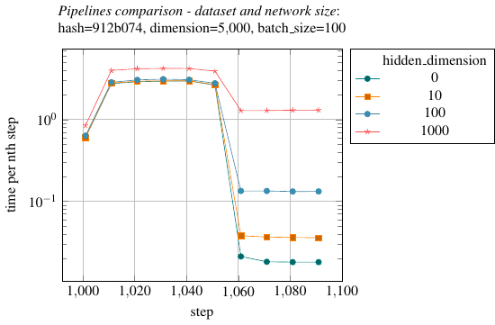
Note that Tensorflow has been designed to use GPU cards such as offered by NVIDIA (and also Google’s own domain-specific chip called Tensor Proccessing Unit). If such a GPU card is employed, the actual linear algebra operations necessary for the gradient calculation and weight and bias updates during training will become negligible except for very large networks (1e6 dof and beyond).
In [references.performance.runtime_comparison_gpu] we give the same runtime profile as before. In contrast to before, the simulation is now done on a system with 2 NVIDIA V100 cards. Comparing this to figure [references.performance.runtime_comparison_cpu] we notice that now all curves associated to different number of nodes in the hidden layer (hidden_dimension) basically lie on top of each other. In the runtime profile on CPUs alone there is a clear trend for networks with more degrees of freedom to significantly require more time per training step. We conclude that with these networks (784 input nodes, 10 output nodes, hidden_dimension hidden nodes, i.e. ~1e6 dof) the V100s do not see full load, yet.
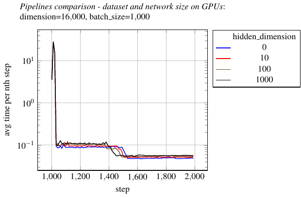
3.9.1. General advice
We conclude this section with some general advice on resolving performance issues:
-
trajectory files become very big with large networks. Do not write the trajectory if you do not really need it. If you do need it, then write only every tenth or better every hundredth step (option every_nth).
-
summaries (option summaries_path) are very costly as well. Write them only for debugging purposes.
-
if you can afford the stochastic noise, use a small batch size (option batch_size).
-
use hessians (option do_hessians) only for really small networks.
-
covariance computations are ${O}(M^2)$ in the number of parameters M. Rather use diffusion_map analysis which is squared only in the number of trajectory steps.
-
measure the time needed for a few sampling/training steps, see the time_per_nth_step in the run info dataframes/files. A very good value is 300 steps per second. If you find you are much worse than this (on otherwise able hardware), then start tweaking parameters.
-
Parallel load is not everything. The dataset pipeline will produce much more parallel load but is not necessarily faster than the in-memory pipeline. The essential measure is steps/second.
-
In case you do not need any extra information such as norm of gradients, noise, momentum, kinetic energy and so forth, then you may set do_accumulates to False (or 0 on the cmd-line). This will deactivate these extra calculations, rendering the associated columns in the averages and run info files/data frames zero. This gives about 20-25% decrease in runtime depending on the network and dataset/batch size.
3.10. Miscellaneous
3.10.1. Displaying a progress bar
For longer simulation runs it is desirable to obtain an estimate after a few steps of the time required for the entire run.
This is possible using the progress option. Specified to 1 or True it will produce a progress bar showing the total number of steps, the iterations per second, the elapsed time since start and the estimated time till finish.
This features requires the tqdm package.
|
Note
|
On the debug verbosity level per output step also an estimate of the remaining run time is given. |
3.10.2. Tensorflow summaries
Tensorflow delivers a powerful instrument for inspecting the inner workings of its computational graph: TensorBoard.
This tool allows also to inspect values such as the activation histogram, the loss and accuracy and many other parameters and values internal to TATi.
Supplying a path /foo/bar present in the file system using the summaries_path variable, summaries are automatically written to the path and can be inspected with the following call to tensorboard.
tensorboard --logdir /foo/bar
The tensorboard essentially comprises a web server for rendering the nodes of the graph and figures of the inspected values inside a web page. On execution it provides a URL that needs to be entered in any web browser to access the web page.
|
Note
|
The accumulation and writing of the summaries has quite an impact on TATi’s overall performance and is therefore switched off by default. |
Acknowledgements
Thanks to all users of the code!
Literature
-
Barzilai, J., & Borwein, J. M. (1988). Two-Point Step Size Gradient Methods. IMA Journal of Numerical Analysis, 8(1), 141–148. http://doi.org/10.1093/imanum/8.1.141
-
Bishop, Christopher M. (2006). Pattern Recognition and Machine Learning. Springer Scienice+Business Media, LLC. https://www.springer.com/de/book/9780387310732
-
Bungartz, H. J., & Griebel, M. (2004). Sparse grids. Acta Numerica, 13, 147–269. http://doi.org/10.1017/S0962492904000182
-
Coifman, R. R., & Lafon, S. (2006). Diffusion maps. Applied and Computational Harmonic Analysis, 21(1), 5–30. https://doi.org/10.1016/j.acha.2006.04.006
-
Duane, S., Kennedy, A. D., Pendleton, B. J., & Roweth, D. (1987). Hybrid Monte Carlo. Physics Letters B, 195(2), 216–222. http://doi.org/10.1016/0370-2693(87)91197-X
-
Goodman, J., & Weare, J. (2010). Ensemble samplers with affine invariance. Communications in Applied Mathematics and Computational Science, 5(1), 65–80. http://doi.org/10.2140/camcos.2010.5.65
-
LeCun, Y., Chopra, S., Hadsell, R., Ranzato, M., & Huang, F. J. (2006). A Tutorial on Energy-Based Learning. Predicting Structured Data, 191–246. http://doi.org/10.1198/tech.2008.s913
-
Leimkuhler, B., & Matthews, C. (2012). Rational Construction of Stochastic Numerical Methods for Molecular Sampling. Applied Mathematics Research EXpress, 2013(1), 34–56. http://doi.org/10.1093/amrx/abs010
-
Leimkuhler, B., Matthews, C., & Stoltz, G. (2015). The computation of averages from equilibrium and nonequilibrium Langevin molecular dynamics. IMA Journal of Numerical Analysis, 1–55. http://doi.org/10.1093/imanum/dru056
-
Mackenzie, P. B. (1989). An improved hybrid Monte Carlo method. Physics Letters B, 226(3–4), 369–371. https://doi.org/10.1016/0370-2693(89)91212-4
-
Matthews, C., Weare, J., & Leimkuhler, B. (2018). Ensemble preconditioning for Markov chain Monte Carlo simulation. Statistics and Computing, 28(2), 277–290. http://doi.org/10.1007/s11222-017-9730-1
-
Neal, R. M. (2011). MCMC Using Hamiltonian Dynamics. In Handbook of Markov Chain Monte Carlo (pp. 113–162).
-
Pflüger, D. (2010). Spatially Adaptive Sparse Grids for High-Dimensional Problems. PhD thesis. Technische Universität München. http://www5.in.tum.de/pub/pflueger10spatially.pdf
-
Shang, X., Zhu, Z., Leimkuhler, B., & Storkey, A. J. (2015). Covariance-Controlled Adaptive Langevin Thermostat for Large-Scale Bayesian Sampling. In C. Cortes and N. D. Lawrence and D. D. Lee and M. Sugiyama and R. Garnett (Ed.), Advances in Neural Information Processing Systems 28 (pp. 37–45). Curran Associates, Inc. http://doi.org/10.1515/jip-2012-0071
-
Tan, C., Ma, S., Dai, Y.-H., & Qian, Y. (2016). Barzilai-Borwein Step Size for Stochastic Gradient Descent, 1–17. Retrieved from http://arxiv.org/abs/1605.04131
-
Trstanova, Z. (2016). Mathematical and Algorithmic Analysis of Modified Langevin Dynamics.
-
Welling, M., & Teh, Y.-W. (2011). Bayesian Learning via Stochastic Gradient Langevin Dynamics. Proceedings of the 28th International Conference on Machine Learning, 681–688. http://doi.org/10.1515/jip-2012-0071
Glossary
-
BAOAB is the short-form for the order of the exact solution steps in the splitting of the Langevin Dynamics SDE: B means momentum update, A is the position update, and O is the random noise update. It has 2nd order convergence properties, showing even 4th order super-convergence in the context of high friction, see [Leimkuhler2012].
-
Covariance Controlled Adaptive Langevin (CCAdL)
This is an extension of [SGD] that uses a thermostat to dissipate the extra noise through approximate gradients from the system.
-
An iterative, first-order optimization that use the negative gradient times a step width to converge towards the minimum.
-
Geometric Langevin Algorithm (GLA)
This family of samplers results from a first-order splitting between the Hamiltonian and the Ornstein-Uhlenbeck parts. It provides up to second-order accuracy. In the package we have implemented both the 1st and 2nd order variant. GLA2nd is among the most accurate samplers, especially when it comes to accuracy of momenta. It is surpassed by BAOAB, particularly for positions.
-
Instead of Langevin Dynamics this sampler relies on Hamiltonian Dynamics. After a specific number of trajectory steps an acceptance criterion is evaluated. Afterwards momenta are drawn randomly. Hence, here noise comes into play at distinct intervals while for the other samplers noise enters gradually in every step.
-
Stochastic Gradient Descent (SGD)
A variant of [GD] where not the whole dataset is used for the gradient computation but only a smaller part. This lightens the computational complexity and adds some noise to the iteration as gradients are only approximate. However, given redundancy in the dataset this noise is often welcome and helps in overcoming barriers in the non-convex minimization problem.
See also [GD].
-
Stochastic Gradient Langevin Dynamics (SGLD)
A variant of SGD where the approximate gradients are not only source of noise but an additional noise term is added whose magnitude controls the noise from the gradients.
See also [SGD].