%matplotlib inlineOther Contributors
- Camila Rangel Smith, Alan Turing Institute, GitHub: @crangelsmith. Twitter: @CamilaRangelS.
- Martin O’Reilly, Alan Turing Institute, Github: @martintoreilly.
Reviewers
- Sam Van Stroud, University College London, GitHub: @samvanstroud
- Kevin Xu, Civil Service Fast Stream, GitHub: @kevinxufs
Introduction
The Covid-19 Pandemic led to record numbers of mail-in votes in the 2020 United States Presidential Election. Because of the high volume of mail ballots, plus rules that prevented some states from counting these ballots before election day, the result of the election remained uncertain for a week, with periodic updates coming as ballots were tabulated and reported.
In particular, several states had very close races that had the potential to tip the election in favor of either candidate. The US elects the president using the Electoral College system, where every state has a fixed number of electoral votes depending on its population. These electoral votes determine the outcome, not the national popular vote. The states almost universally employ a “winner-take-all” model for allocating their electoral votes. Because of this, each year a few “swing states” have a large effect on the outcome of the election. For example, in 2000 the election came down to around a 500 vote margin in Florida (out of over 6 million ballots cast), despite the fact that Al Gore easily won the national popular vote. In 2020, a few states with very close races dominated the headlines for the week after the election, of which we will look at Pennsylvania, Arizona, and Georgia in this post. The final outcome of the election hung on the results from these states, and the slow drip feed of additional ballots being released left the public constantly checking the news for updates.
In this Turing Data Story, I examine a few ways to analyze the data updates coming from each state to predict the final outcome. This originated from some Slack discussions with Camila Rangel Smith and Martin O’Reilly, whom I list above as contributors for this reason. In particular, our initial interest in this question centered around uncertainties in the analysis done by Camila and Martin, which I have carried out using Bayesian inference to quantify uncertainty and determine when we might have reasonably called each state for the eventual winner based on the data as it underwent regular updates.
Data
To create the models in the post, I use the NYT Election Data Scraper, which is an open source repository that collected data from the New York Times website every few minutes over the months following the election. We can use this data to explore how the results evolved over time following election day, and compare our results with how the news media reported these changes over time.
In particular, the data includes an estimate of the number of votes remaining, which is a crucial figure that we need in order to mathematically forecast the outcome. The New York Times bases their model for the votes remaining using turnout estimates from Edison Research, which is mentioned here. Based on this turnout estimate, combined with the updates of votes as they are counted, we can use this data to forecast the outcome.
To load this data into a Python session for analysis, I can use Pandas to simply load from the CSV version of the data directly from the URL, and extract the state that I wish to examine:
import pandas
import datetime
def load_data(state, timestamp=None):
"""
Loads election data updates from CSV file as a pandas data frame
Retrieves data from the live file on Github, which is loaded into a
data frame before extracting the relevant state data.
State must be a string, which will be searched in the "state" field
of the data frame.
Timestamp must be a datetime string. Optional, default is current
date and time.
Returns a data frame holding all updates from a particular state,
prior to the given timestamp. The "vote_differential" field is turned
into a signed margin that is positive for a Biden lead. Also adds
columns for the number of votes for Biden and Trump.
"""
if timestamp is None:
timestamp = datetime.datetime.now().strftime("%Y-%m-%dT%H:%M:%S")
try:
data = pandas.read_csv("https://alex.github.io/nyt-2020-election-scraper/battleground-state-changes.csv")
except:
data = pandas.read_csv("battleground-state-changes.csv")
data.loc[data["leading_candidate_name"] == "Trump", "vote_differential"] \
= -data.loc[data["leading_candidate_name"] == "Trump", "vote_differential"]
data["biden_votes"] = None
data.loc[data["leading_candidate_name"] == "Biden", "biden_votes"] \
= data.loc[data["leading_candidate_name"] == "Biden", "leading_candidate_votes"]
data.loc[data["trailing_candidate_name"] == "Biden", "biden_votes"] \
= data.loc[data["trailing_candidate_name"] == "Biden", "trailing_candidate_votes"]
data["trump_votes"] = None
data.loc[data["leading_candidate_name"] == "Trump", "trump_votes"] \
= data.loc[data["leading_candidate_name"] == "Trump", "leading_candidate_votes"]
data.loc[data["trailing_candidate_name"] == "Trump", "trump_votes"] \
= data.loc[data["trailing_candidate_name"] == "Trump", "trailing_candidate_votes"]
data["timestamp"] = pandas.to_datetime(data["timestamp"])
data = data[data["timestamp"] < pandas.to_datetime(timestamp)]
return data[data["state"].str.contains(state)]Note that rather than specifying the leading and trailing candidates, I instead just convert the vote differential into a margin that is positive if Biden is leading and negative if Trump is leading. I also add columns for the total number of votes for Biden and Trump, which I will use later.
For instance, if I would like to see the data for Georgia:
df = load_data("Georgia")
df.head()| state | timestamp | leading_candidate_name | trailing_candidate_name | leading_candidate_votes | trailing_candidate_votes | vote_differential | votes_remaining | new_votes | new_votes_relevant | ... | trailing_candidate_partition | precincts_reporting | precincts_total | hurdle | hurdle_change | hurdle_mov_avg | counties_partition | total_votes_count | biden_votes | trump_votes | |
|---|---|---|---|---|---|---|---|---|---|---|---|---|---|---|---|---|---|---|---|---|---|
| 112 | Georgia (EV: 16) | 2020-12-07 20:17:22.360 | Biden | Trump | 2473633 | 2461854 | 11779 | -2224 | -8 | 1 | ... | 75.000000 | 2655 | 2655 | 0.0 | 0.0 | 0.360367 | {} | 4997716 | 2473633 | 2461854 |
| 113 | Georgia (EV: 16) | 2020-12-05 00:26:57.152 | Biden | Trump | 2473707 | 2461779 | 11928 | -2232 | -842 | -858 | ... | 0.067599 | 2655 | 2655 | 0.0 | 0.0 | 0.368200 | {'Appling': 49, 'Ben Hill': 4, 'Bleckley': 2, ... | 4997724 | 2473707 | 2461779 |
| 114 | Georgia (EV: 16) | 2020-11-20 22:11:31.395 | Biden | Trump | 2474507 | 2461837 | 12670 | -3074 | -954 | -917 | ... | 0.214831 | 2655 | 2655 | 0.0 | 0.0 | 0.364533 | {} | 4998566 | 2474507 | 2461837 |
| 115 | Georgia (EV: 16) | 2020-11-20 21:57:11.453 | Biden | Trump | 2475227 | 2462034 | 13193 | -4028 | -770 | -532 | ... | 0.855263 | 2655 | 2655 | 0.0 | 0.0 | 0.349900 | {} | 4999520 | 2475227 | 2462034 |
| 116 | Georgia (EV: 16) | 2020-11-20 21:51:12.226 | Biden | Trump | 2475304 | 2462489 | 12815 | -4798 | -1958 | -1851 | ... | 0.518098 | 2655 | 2655 | 0.0 | 0.0 | 0.356867 | {} | 5000290 | 2475304 | 2462489 |
5 rows × 22 columns
The data contains a timestamp, the number of votes for each candidate, the margin, and an estimate of the number of votes remaining. Note that because the number of votes remaining is just an estimate, it can eventually become negative if the eventual number of ballots exceeds the estimate used to forecast the number of remaining votes. We can also have situations where the number of votes is corrected downwards, so we will need to take care that these do not trip up our model.
When the data is captured in this way, we can see how the vote margin evolves over time as new ballots are counted. For example, we can look at the data for all states up to midnight on 5 November to see the evolution of the race:
import matplotlib.pyplot as plt
state_list = ["Pennsylvania", "Georgia", "Arizona"]
timestamp_list = ["2020-11-05T00:00:00"]*3
iter_vals = list(zip(state_list, timestamp_list))
def plot_data(state, timestamp=None):
"Plot the election data for a given state up through a given time"
df = load_data(state, timestamp)
plt.figure()
plt.plot(df["votes_remaining"], df["vote_differential"], "o")
plt.xlabel("Votes remaining")
plt.ylabel("Biden margin")
plt.title("{} Vote Updates through {}".format(state, timestamp))
for (state, tstamp) in iter_vals:
plot_data(state, tstamp)
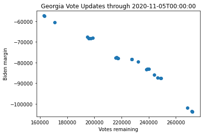
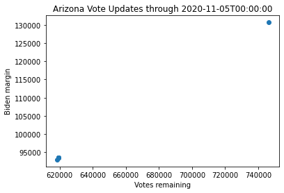
Note that the trend shows that Biden is catching up as more votes are counted in both Georgia and Pennsylvania, while Trump is catching up in Arizona. The trend is fairly linear. Thus, one might first consider doing a simple regression to estimate the final margin.
Linear Regression Analysis
As a first pass at building a model, I can do a simple regression analysis. A linear regression model will have two parameters that are fit: the slope will be related to the fraction of the outstanding votes that are for Biden, and the intercept, which will indicate the final margin when there are no votes remaining. (This is the initial analysis that was done by Camila for Pennsylvania and Martin for Arizona.)
import numpy as np
def linear_regression(state, timestamp=None):
"""
Fit a linear regression model to the election updates
Fits a line to the data updates for a given state and a given
timestamp. Plots the data and returns the fitting parameters
(slope, intercept) as a numpy array.
"""
plot_data(state, timestamp)
df = load_data(state, timestamp)
coeffs = np.polyfit(df["votes_remaining"], df["vote_differential"], 1)
plotvals = np.linspace(0, df["votes_remaining"].iloc[-1])
plt.plot(plotvals, coeffs[0]*plotvals + coeffs[1])
return coeffs
for (state, tstamp) in iter_vals:
coeffs = linear_regression(state, tstamp)
print("Predicted margin for {} as of {}: {}".format(state, tstamp, coeffs[1]))Predicted margin for Pennsylvania as of 2020-11-05T00:00:00: 139881.65460479335
Predicted margin for Georgia as of 2020-11-05T00:00:00: 11362.338299788926
Predicted margin for Arizona as of 2020-11-05T00:00:00: -87876.90143040325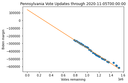
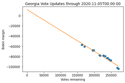
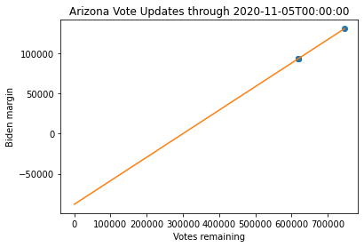
Note that at this point, the linear regression predicts a margin in Pennsylvania and Arizona that are quite different from the final margin. Georgia appears to be very close to the final margin. However, Arizona seems to have outlier points that muddles this analysis (which was first noted by Martin). Thus, while these models are useful starting points, they do not appear to be particularly robust and are somewhat dependent on when you choose to fit the data.
def get_margin(state, timestamp=None):
"Extract margin for a state at a given time"
df = load_data(state, timestamp)
return df["vote_differential"].iloc[0]
for state in state_list:
print("Current margin in {}: {}".format(state, get_margin(state)))Current margin in Pennsylvania: 81660
Current margin in Georgia: 11779
Current margin in Arizona: 10457However, one thing to note about this is that even though the trends point clearly in favor of Biden in this analysis, we do not have a good idea of the uncertainties. Without an uncertainty, we cannot robustly evaluate if the model is making good predictions. How might we develop a model that explicitly captures this uncertainty? And given such a model, when can we be confident that a candidate has won the state, and how does it align with the narrative from the news media? The following describes one approach for doing so.
Modelling Uncertainty in the Votes
To address this shortcoming, we turn to Bayesian Inference. Bayesian statisticians think of model parameters not as a single number, but rather probability distributions – in this way, we can get a sense of the range of values that the model thinks are consistent with the data.
Model Structure
As noted above, the regression model has two different parameters: the slope (related to the fraction of votes that are cast for Biden), and the intercept (which is essentially the prediction of the final margin). Note that while the linear regression fit these two things simultaneously, there is no reason why I had to let the final margin be a “free” parameter that was adjusted in the fitting: I could have instead just fit a single parameter for the slope (for instance, simply using the fraction of mail ballots cast thus far for one of the candidates), and then used that estimate to project the votes remaining in order to extrapolate and obtain an estimate of the final margin.
We would like to adjust our model to account for uncertainty in both of these pieces of the model. The main source of uncertainty in the vote probability is related to the fact that not all voters are identical – the regression model assumes that this is the case, and the main challenge in building a more complex model is to relax this constraint while still ensuring that the model is simple enough that we can reliably fit it with the available data. For this, I will propose what is known as a hierarchical model, which is a common way of adding more complexity to a model in Bayesian inference. However, this is not the only way to do this, and there are certainly other methods based on Bayesian inference that would be able to account for this type of uncertainty.
There is also some uncertainty to account for in projecting the remaining votes, but it turns out that this is much smaller than the uncertainty in the vote probability. The way that I handle this type of uncertainty is a fairly standard problem in Bayesian inference, so I will focus most of my attention here on how to make a model that does not treat all voters identically, as this is the principal source of uncertainty. The following sections outline how to build such a model, fit its parameters, and then project the election outcome once it has been fit.
Bayesian Model of the Vote Probability
Bayesian inference tends to think of probability distributions as reflecting statements about our beliefs. Formally, I need to state my initial beliefs before I see any data, and then I can use that data to update my knowledge. This previous belief is known as a prior in Bayesian inference, and the updated beliefs once I look at the data is known as the posterior.
Bayesian Inference
Bayesian inference involves taking our previous beliefs about a system, described by a probability distribution of reasonable values we expect a particular parameter to take, and then using the data to update those beliefs about the distribution that we expect that parameter to take by computing the posterior. A key concept in Bayesian statistics is the idea of a conditional probability, written \(p(A|B)\), which means the probability of \(A\) given that we already know \(B\) (or conditioned on \(B\)). Inference allows us to update our beliefs (or in other words condition them on something we have observed) by applying Bayes’ rule:
\[ p(\theta|y) = \frac{p(y|\theta)p(\theta)}{p(y)} \]
Here, \(p(\theta)\) is the prior distribution (which we will specify before looking at the data), \(p(y|\theta)\) is the likelihood (the probability that we would have gotten the data conditioned on a particular value of \(\theta\)), and \(p(y)\) is known as the evidence (the probability of getting that particular observation over all possible outcomes of the experiment). Note that we have two standard probability distributions (the prior and the evidence), and two conditional probabilities (the likelihood and the posterior). The one we really care about is the posterior (our belief in the model parameters conditioned on the data, since the model parameters are uncertain but the data is known), but in practice it is much easier to compute the likelihood; Bayes’ rule tells us how these two are connected and makes these kind of computations more practical.
In practice, for most models one cannot compute the evidence very easily, so instead of computing the posterior directly, one draws samples from it. A common technique for this is Markov Chain Monte Carlo (MCMC) sampling. A number of software libraries have been written in recent years to make carrying out this sampling straightforward using what are known as probabilistic programming languages. These languages formally treat variables as probability distributions with priors and then draw samples from the posterior to allow the user to more easily perform inference.
Note that because I will ultimately draw samples from the posterior, rather than compute the probability density function itself, most of the plots in this story will not have meaningful vertical axis scales, as the scale will depend on the number of samples that were drawn. Thus in most cases I simply omit labels on the vertical axes, as these are implicitly the number of samples in each case.
A Hierarchical Bayesian Model For Voting
In the linear regression model, we effectively treat the vote probability as a single, unchanging value. This is the same as saying that every voter in our model is identical. Given the political polarization in the US, this is probably not a very good assumption. Although the data seems to strongly suggest that the mail-in votes are consistently in favor of one candidate, this is not the same as saying all voters are identical. In the following, I build a model to relax this assumption, using what is known as a hierarchical Bayesian model.
If the above model of assuming that every voter is identical is one extreme, then the other extreme is to assume that every voter is different and we would need to estimate hundreds of thousands to millions of parameters to fit our model. This is not exactly practical, so a hierarchical model posits a middle ground that the vote probability is itself drawn from a probability distribution. In this manner, we can use a probability distribution to describe the overall population of voters, and thus rather than fitting a parameter for every single voter, we just need to fit a few parameters to specify the distribution.
This structure is why hierarchical models are so powerful: probability distributions can be described with only a small number of parameters, so they are easy to fit, but we will see that it vastly expands the range of outcomes that the model is able to produce. This is in essence why hierarchical models can be so powerful – they guard against overfitting by using only a few parameters, but they can still produce a large variety of outcomes.
In the following, we model the vote probability by assuming that each vote update has a single vote probability associated with it, and that vote probability is drawn from a beta distribution. A beta distribution is a distribution defined over the interval \([0,1]\) with two shape parameters \(a\) and \(b\) that lets us flexibly specify a wide range of outcomes. If \(a\) and \(b\) are less than 1, then the distribution is biased towards the extreme values of 0 or 1, while if they are greater than 1 then the distribution is biased towards 0.5. If \(a > b\), then the model is more biased towards 1, while if \(b > a\) then the model is biased towards 0. Thus we can specify a huge range of distributions with just two parameters.
from scipy.stats import beta
def plot_beta(a, b):
"Plot the beta distribution for shape paramters (a, b)"
xvals = np.linspace(0, 1)
plt.plot(xvals, beta.pdf(xvals, a=a, b=b))
plt.xlabel("Biden vote probability")
plt.title("PDF for the Beta distribution with a = {}, b = {}".format(a, b))
plot_beta(8., 4.)
Thus, instead of estimating the vote probability, I instead need to estimate \(a\) and \(b\), which will tell us what I expect the distribution of the vote probability to be. Having multiple levels of distributions described by distributions like this are what give hierarchical models their name – parameters are drawn from distributions, and this distribution must be described by some parameters. But because all parameters in Bayesian inference are probability distributions, these parameters are also distributions themselves, hence the model is hierarchical.
Since all parameters in a Bayesian model must have priors, our task is now to encode our prior beliefs about the vote probability distribution by setting prior distributions for \(a\) and \(b\).
Prior
The prior represents our previous beliefs about the value of the model parameters before we see any data, or in other words what we expect to be reasonable. If you are observing outcomes from flipping a coin, you might reasonably expect the probability of getting heads to be close to 0.5 in the absence of any data, and you might be unwilling to accept the idea of this probability of being 0 or 1. This is encoded in a probability distribution function, usually by using a particular distribution that is convenient given the constraints of the particular problem (for instance, the beta distribution described above is one that is often used to model priors where the parameter in question is a probability).
Often, in Bayesian inference one does not have strong feelings about what values they might expect for a parameter. In those cases, we might prefer to use something simple, what is known as an uninformative prior. These might be expressed as a statement like “every value is equally probable”. Or in this case we might assume that the prior for the vote probability should be peaked close to 0.5, and then taper off towards 0 and 1, with the argument that US presidential elections are usually decided by a few percentage points difference in the national popular vote. This might seem very reasonable on the surface, as America is pretty evenly divided between Democrats and Republicans.
However, mail in votes in practice can be extremely biased towards one party. Historically, a large majority of mail in ballots are Democratic, for a variety of reasons that are largely demographic. Trump also spent much of the campaign sowing doubt about mail-in ballots (telegraphing his post-election strategy of trying to throw them out in court), so his supporters may be much less likely to vote in this manner. However, there could also be a situation where the mail-in ballots fall heavily towards a Republican candidate (as we have seen already, more of the Arizona ballots tend to be in favor of Trump, which was due to late arriving ballots being from Republicans that registered to vote just before the election). Thus, based on this I would argue that what we actually want is a prior that is reasonably likely to include some extremes in the vote probability to ensure that our estimate of the final outcome prior to looking at the data doesn’t exclude a significant swing.
This issue illustrates a challenge with Bayesian Hierarchical models – when the parameter that I have some knowledge about is itself described by a distribution, the priors for the distribution parameters can be more difficult to specify. For this reason, modellers often go one level further and specify prior distributions on the parameters used to specify the priors on the model parameters, which are known as hyperpriors, and see how varying the priors changes the outcome of inference. I will not explore this level of Bayesian modelling, but in building this model I had to try a number of different choices for the priors before arriving at something that I thought accurately reflected my prior beliefs about the outcome.
In the priors that I finally settled on, I use a Lognormal distribution for my prior on \(a\) and \(b\). Lognormal distributions are frequently used as an alternative to a normal distribution in situations when the parameter in question must be positive (effectively, lognormal distributions can thought of as having the logarithm of the random variable in question following a normal distribution). I choose the parameters of the lognormal distributions for \(a\) and \(b\) to be slightly different such that the resulting distributions are more likely to lean democratically (as mail in votes are historically more democratic leaning), but still have a decent chance of producing extremes for Trump. I also choose the parameters such that I get a mix of values more biased towards the extremes as well as those biased towards values closer to 0.5.
Priors like the ones used here are often referred to as subjective priors. Depending on who you ask, this is either a strength or a weakness in Bayesian inference. On one hand, the results are somewhat dependent on my parameter choices for my priors, but on the other hand, nearly every scientific study reflects some of the biases of the researchers that carry out the work. Subjective priors have the benefit of explicitly codifying the assumptions I made about what I expect to be reasonable outcomes, at the cost of some potential subjectivity in the final results. In this era of significant divides across party lines, exposing this part of the model as inherently subjective may also help ensure that the model parameters are not chosen in a way that explicitly favors one party over another.
As we will see, using this prior allows for the possibility that there is a decent chance based on historical data that the mail votes are heavily in favor of one candidate. The parameters I choose give a slight edge to the candidate from the Democratic party, but the prior includes a very reasonable chance that the swings will be towards the Republican candidate, which should help ensure that the model is not perceived to be biased against either candidate. Here are some histograms showing single samples of the vote probability drawn from this prior, and an aggregate histogram of 100 samples:
from pymc3 import Lognormal
def plot_prior_samples(n_samples):
"Plot a random draw of the vote probability from the prior"
a = Lognormal.dist(mu=0.4, sd=0.5).random(size=n_samples)
b = Lognormal.dist(mu=0.2, sd=0.5).random(size=n_samples)
x = np.linspace(0., 1.)
plt.figure()
plt.hist(beta.rvs(size=(1000, n_samples), a=a, b=b).flatten(), bins=100)
plt.xlabel("Biden vote probability")
plt.title("Prior Vote Probability Distribution using {} samples".format(i))
for i in [1, 1, 1, 100]:
plot_prior_samples(i)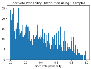
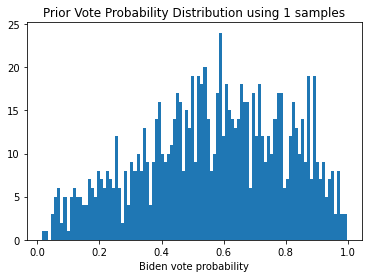

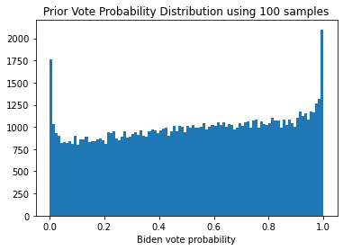
From these individual samples, as well as the aggregated histogram, we see that we get a range of outcomes, with a slight bias towards those that favor democrats. As we acquire enough data to reliably estimate the underlying distribution of the vote probabilites, we should see better estimates of the true distribution, which will eliminate more of the extremes and reduce the uncertainty in the final outcome.
Likelihood
Finally, we need to explicitly model the likelihood. The likelihood is how Bayesian models connect the parameters to the data – the likelihood tells us how probable the data is conditioned on a particular choice of parameters. As discussed earlier, this is actually the opposite of what we want, as we are interested in the parameters conditioned on the data. However, Bayes’ rule helps us compute the quantity we are interested in as long as we are able to to compute the likelihood.
For this particular problem, we can fortunately compute the likelihood easily in closed form. When one flips a fair coin a number of times, the distribution of outcomes follows a binomial distribution. Thus, I can use a binomial likelihood to model the range of vote probabilites that might be consistent with the votes that were cast. This can be computed analytically, and most probabilistic programming languages have built-in capacity for computing likelihoods of this type (so that we don’t have to worry about writing down the correct formula and implementing and testing the code to do this ourselves!). This is done automatically when using a probabilistic programming language by setting this particular variable to have a known value, which indicates to the probabilistic programming language that this variable is used to compute the likelihood. This means that I can focus on describing the model, rather than how to do the computation, which is one of the strengths of this type of modelling.
PyMC3 Implementation
Thus, I can now write down a model in a probabilistic programming language in order to draw samples from the posterior. There are a number of popular lanaguages for this – here I use PyMC3 to implement my model. PyMC3 can easily handle all of the features I specified above (hierarchical structure, and a binomial likelihood), which is written out in the function below.
In coding up the model, I need to convert the election data into a series of “trials” consisting of a number of total votes cast and the corresponding number of votes for Biden. This is the way that the information needs to be captured to compute the binomial likelihood, which can then be used to draw samples from the posterior. Earlier, I noted that the data sometimes contains some inconsistencies (i.e. there are more votes cast for one candidate than the total number in that batch), so to protect against this I perform some checks for consistency and throw out any data that doesn’t make sense (in particular, I want to be sure the total number of votes is non-negative and the number of votes cast for Biden is smaller than the total number of ballots in this particular batch). I do this using a Numpy logical array in the extract_vote_trials function, as otherwise some inconsistent data can trip up the PyMC computations.
Once we have the trials defined, we can specify our model using PyMC3, perform inference, and plot the results:
import pymc3
import logging
logger = logging.getLogger("pymc3")
logger.propagate = False
logger.setLevel(logging.ERROR)
def extract_vote_trials(state, timestamp=None):
"""
Convert vote data into a series of bernoulli trials. If no
data is valid (i.e. check that all numbers are nonzero and
the number of total ballots cast is larger than the number
of votes for, then return a list of a single zero for each.
Returns two lists of positive integers for the total number
of votes and the votes for Biden
"""
df = load_data(state, timestamp)
total_votes = np.diff(-df["biden_votes"]) + np.diff(-df["trump_votes"])
biden_votes = np.diff(-df["biden_votes"])
# throw out combinations that don't make any sense using numpy
# logical arrays -- note that multiplication of logical arrays
# is equivalent to a logical "and";
# if none remain then just return (0,0)
trials_to_keep = ((total_votes > 0)*(biden_votes >= 0)*
(biden_votes <= total_votes))
total_votes = total_votes[trials_to_keep]
biden_votes = biden_votes[trials_to_keep]
if len(total_votes) == 0:
total_votes = [0]
biden_votes = [0]
return (np.array(total_votes, dtype=np.int64),
np.array(biden_votes, dtype=np.int64))
def estimate_theta_hierarchical(state, timestamp=None):
"Estimate the vote probability distribution using a hierarchical model and MCMC sampling"
total_votes, biden_votes = extract_vote_trials(state, timestamp)
num_trials = len(total_votes)
# build model and draw MCMC samples
with pymc3.Model() as model:
a = pymc3.Lognormal("a", mu=0.4, sd=0.5)
b = pymc3.Lognormal("b", mu=0.2, sd=0.5)
theta = pymc3.Beta("theta", alpha=a, beta=b, shape=num_trials)
obs = pymc3.Binomial("obs", p=theta, n=total_votes,
observed=biden_votes, shape=num_trials)
trace = pymc3.sample(1000, progressbar=False,
return_inferencedata=False)
return trace
def plot_posterior(state, timestamp):
"Plot the posterior distribution of the vote probability"
trace = estimate_theta_hierarchical(state, timestamp)
rvs_size = (100, len(trace["a"]))
plt.figure()
plt.hist(beta.rvs(size=rvs_size,
a=np.broadcast_to(trace["a"], rvs_size),
b=np.broadcast_to(trace["b"], rvs_size)).flatten(),
bins=100)
plt.xlabel("Biden vote probability")
plt.title("{} Vote Probability Posterior as of {}".format(state, timestamp))
for (state, tstamp) in iter_vals:
plot_posterior(state, tstamp)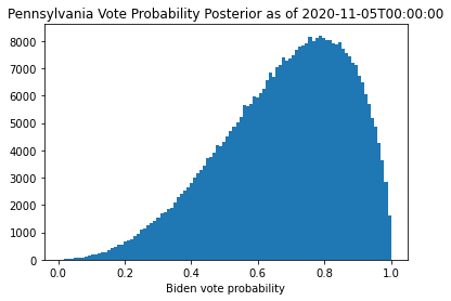
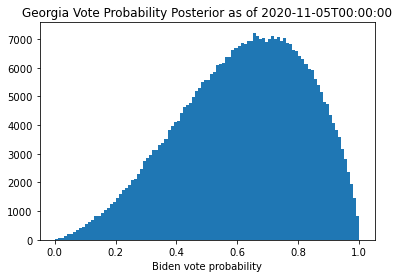

Once I draw MCMC samples for \(a\) and \(b\), I convert those samples into samples of \(\theta\) to see our posterior estimate of the vote probability.
Looking at these plots, I see that the model is now much more varied in its estimates for the vote probability (note that this is the posterior for the distribution expected for the vote probability, rather than the explicit values of the vote probability itself). The mean is still where I expect it based on the linear regression analysis, but the distribution is much wider due the fact that occasionally votes come in from places that are not as heavily in favor of Biden (or Trump in the case of Arizona). This wider distribution of the vote probability is how I quantify the larger uncertainty in the election outcome. Using this distribution to forecast the remaining votes should considerably increase the spread of the predicted final margin and assure that it is not overconfident in the final result.
Predicting the Final Margin
Once I have samples from the vote probability, I need to simulate the remaining votes to predict the final outcome. This is known as estimating the posterior predictive distribution in Bayesian inference, when one uses the updated knowledge about one of the model parameters to predict something that was not used to fit the data.
What is a reasonable way to simulate the remaining votes? As one can see from the data, the votes come in a steady drip feed as ballots are counted. Thus, I can simulate this by sampling randomly, with replacement, from the data for the number of ballots cast in each update until I get to the number of votes remaining. I can then use the posterior samples of \(a\) and \(b\) to generate a distribution of vote probabilities, and then draw from the vote probabilites to forecast the outcome of each batch of votes using a binomial distribution. I repeat this process 10 times to ensure that the result isn’t dependent on the particular realization of the drip feed simulation, and aggregate those samples to get the final estimate of the posterior predictive distribution. This should give a reasonable estimate of the final outcome based on the model.
from scipy.stats import binom
def get_votes_remaining(state, timestamp=None):
"Extract remaining votes for a state at a given timestamp"
df = load_data(state, timestamp)
return df["votes_remaining"].iloc[0]
def draw_random_vote_updates(state, timestamp):
"Draw a random set of simulated vote updates for the remaining votes"
n_remain = get_votes_remaining(state, timestamp)
n, k = extract_vote_trials(state, timestamp)
if np.all(n == 0):
n = np.array([1000], dtype=np.int64)
simulated_vote_updates = []
while np.sum(simulated_vote_updates) <= n_remain:
simulated_vote_updates.append(np.random.choice(n))
simulated_vote_updates[-1] = n_remain - np.sum(simulated_vote_updates[:-1])
assert np.sum(simulated_vote_updates) == n_remain
return np.array(simulated_vote_updates, dtype=np.int64)
def project_remaining_votes(trace, simulated_vote_updates):
"Project the remaining votes using MCMC samples of the vote probability distribution parameters"
assert np.all(trace["a"] >= 0.)
assert np.all(trace["b"] >= 0.)
rvs_size = (len(trace["a"]), len(simulated_vote_updates))
return np.sum(binom.rvs(size=rvs_size,
p=beta.rvs(size=rvs_size,
a=np.broadcast_to(trace["a"][:, np.newaxis], rvs_size),
b=np.broadcast_to(trace["b"][:, np.newaxis], rvs_size)),
n=np.broadcast_to(simulated_vote_updates, rvs_size)), axis=-1)
def predict_final_margin(trace, state, timestamp=None):
"""
Use posterior samples of the vote probability to predict the remaining
votes.
The remaining votes are split into batches by sampling from
the previous votes until enough are accumulated. Then each batch is
forecast using the posterior samples, and the total is summed.
Returns a numpy array of samples of the final margin
"""
# simulate remaining votes
n_trials = 10
predicted_margin = np.zeros((n_trials, len(trace["a"])))
for i in range(n_trials):
simulated_vote_updates = draw_random_vote_updates(state, timestamp)
predicted_margin[i] = project_remaining_votes(trace, simulated_vote_updates)
n_remain = get_votes_remaining(state, timestamp)
margin = get_margin(state, timestamp)
return margin - n_remain + 2*predicted_margin.flatten()
def plot_predictions(state, timestamp):
"Plot the posterior predictive distribution for the given state and time"
trace = estimate_theta_hierarchical(state, timestamp)
predicted_margin = predict_final_margin(trace, state, timestamp)
plt.figure()
plt.hist(predicted_margin, bins=100)
plt.xlabel("Biden Margin")
plt.title("{} final predicted margin as of {}".format(state, timestamp))
for (state, tstamp) in iter_vals:
plot_predictions(state, tstamp)
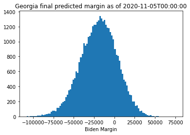
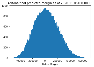
As we can see from this, the model has fairly wide intervals surrounding the predicted final margin based on the original linear regression model. Interestingly, when I fit Georgia in this way, it looks much more likely that Trump would win through this point than the linear regression model would suggest, though the final margin found by the regression analysis is well within the error bounds suggested from the predictions. Arizona looks up for grabs, indicating that the outlier points were definitely biasing the regression analysis. Pennsylvania is much more firmly leaning towards Biden. We can look at the results again a day later to see how the race evolved:
for (state, tstamp) in zip(state_list, ["2020-11-06T00:00:00"]*3):
plot_predictions(state, tstamp)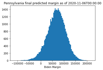
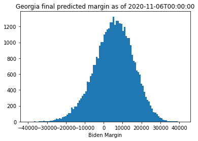
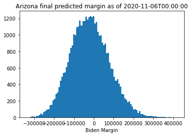
Clearly, Georgia has swung in Biden’s favor over the course of the day. The mean final margin in Pennsylvania has not moved much, though the uncertainty has tightened up and made the result more likely for Biden. Arizona could still go either way.
Animating the Updates
Now that I have built a model, I can build an animation that shows the evolution of the predicted results as a function of time. This will show how the uncertainty shrinks over time as fewer votes remain. I check for results every 30 minutes for the 12 days from 4 November onward, and update the model when new ballots are found. I also compute a Biden win probability and show the mean margin \(\pm\) 2 standard deviations to give an idea of the equivalent regression result and its uncertainty. Building the animation requires some more clever manipulation of Matplotlib objects, so I will not go into detail to describe exactly what the plotting code is doing here. It is based on the code in this example, so please look at that example for a description of how to animate histograms.
Note: Because new MCMC samples need to be drawn for each new update, creating this animation ends up being fairly expensive to run (this took several hours on my laptop). I speed things up by saving the current prediction each time the MCMC samples are drawn, so that if the previous iteration is the same we do not need to re-run the model. However, this is still fairly expensive, so don’t try and run this unless you are willing to wait!
%%capture
import matplotlib.path as path
import matplotlib.patches as patches
import matplotlib.text as text
import matplotlib.animation as animation
def load_previous_model(filename, initialize=False):
"""
Load the previous model from file
Load results from the previous simulation from disk,
including the total votes cast, votes for Biden,
number of votes remaining, and the previous set of
samples from the predictive distribution.
If the file cannot be loaded, or if we pass
`initialize=True`, returns `None` for all values.
"""
total_votes = None
biden_votes = None
n_remain = None
preds = None
if not initialize:
try:
model = np.load(filename)
total_votes = model["total_votes"]
biden_votes = model["biden_votes"]
n_remain = int(model["n_remain"])
preds = model["preds"]
except (KeyError, IOError):
total_votes = None
biden_votes = None
n_remain = None
preds = None
return total_votes, biden_votes, n_remain, preds
def fit_model(state, timestamp=None, initialize=False):
"""
Fit a model to predict the final margin for the given date/time.
Each iteration is saved as a numpy file, and the next step
checks for a model that matches the existing vote count before
doing the expensive MCMC fitting
Returns the simulated final margin samples at the given time
"""
filename = "model.npz"
total_votes_prev, biden_votes_prev, n_remain_prev, preds_prev = \
load_previous_model(filename, initialize)
total_votes, biden_votes = extract_vote_trials(state, timestamp)
n_remain = get_votes_remaining(state, timestamp)
if (np.array_equal(total_votes_prev, total_votes) and
np.array_equal(biden_votes_prev, biden_votes) and
n_remain_prev == n_remain):
return preds_prev
else:
theta = estimate_theta_hierarchical(state, timestamp)
preds = predict_final_margin(theta, state, timestamp)
np.savez(filename,
total_votes=total_votes, biden_votes=biden_votes,
preds=preds, n_remain=n_remain)
return preds
def initialize_verts(bins):
"Initialize the patch corners for the animation"
# get the corners of the rectangles for the histogram
left = bins[:-1]
right = bins[1:]
vals = np.zeros(len(left))
nrects = len(left)
nverts = nrects * (1 + 3 + 1)
verts = np.zeros((nverts, 2))
codes = np.full(nverts, path.Path.LINETO)
codes[0::5] = path.Path.MOVETO
codes[4::5] = path.Path.CLOSEPOLY
verts[0::5, 0] = left
verts[0::5, 1] = vals
verts[1::5, 0] = left
verts[1::5, 1] = vals
verts[2::5, 0] = right
verts[2::5, 1] = vals
verts[3::5, 0] = right
verts[3::5, 1] = vals
return verts, codes
def update_verts(preds, bins, verts):
"Update the verticies on the histogram patches for animation"
n, bins = np.histogram(preds, bins)
verts[1::5, 1] = n
verts[2::5, 1] = n
return verts
def animate(i, state, start_time, bins_t, verts_t, patch_t, bins_b, verts_b, patch_b,
date_text, vote_text, mean_text, prob_text):
"Updates the histogram patches and text to make the animated histogram plot"
hours = i//2
minutes = 30*i % 60
timestamp = ((datetime.datetime.strptime(start_time, "%Y-%m-%dT%H:%M:%S") +
datetime.timedelta(hours=hours, minutes=minutes)).strftime("%Y-%m-%dT%H:%M:%S"))
if i == 0:
preds = fit_model(state, timestamp, initialize=True)
else:
preds = fit_model(state, timestamp)
verts_t = update_verts(preds, bins_t, verts_t)
verts_b = update_verts(preds, bins_b, verts_b)
date_text.set_text(datetime.datetime.strptime(timestamp, "%Y-%m-%dT%H:%M:%S").strftime("%Y-%m-%d %H:%M"))
n_remain = get_votes_remaining(state, timestamp)
vote_text.set_text("{} Votes Remaining".format(str(n_remain)))
mean_text.set_text("Margin = {:>8} $\pm$ {:>7}".format(int(np.mean(preds)),
int(2.*np.std(preds))))
prob_text.set_text("Biden win prob = {:.2f}".format(np.sum(preds > 0)/len(preds)))
return [patch_t, patch_b, date_text, vote_text, mean_text, prob_text]
def create_animation(state):
"Create an animation of the vote updates for the given state"
start_time = "2020-11-04T14:00:00"
xlim = 100000
ylim = 500
nbins = 200
binsize = xlim//nbins
bins_b = np.linspace(0, xlim, binsize, dtype=np.int64)
bins_t = np.linspace(-xlim, 0, binsize, dtype=np.int64)
verts_t, codes_t = initialize_verts(bins_t)
verts_b, codes_b = initialize_verts(bins_b)
patch_t = None
patch_b = None
fig, ax = plt.subplots()
barpath_t = path.Path(verts_t, codes_t)
patch_t = patches.PathPatch(barpath_t, facecolor='C3',
edgecolor='C3', alpha=0.5)
ax.add_patch(patch_t)
barpath_b = path.Path(verts_b, codes_b)
patch_b = patches.PathPatch(barpath_b, facecolor='C0',
edgecolor='C0', alpha=0.5)
ax.add_patch(patch_b)
lefttext = -9*xlim//10
righttext = 9*xlim//10
uppertext = 9*ylim//10
lowertext = 8*ylim//10
date_text = text.Text(lefttext, uppertext, "")
ax.add_artist(date_text)
vote_text = text.Text(lefttext, lowertext, "")
ax.add_artist(vote_text)
prob_text = text.Text(righttext, uppertext, "", ha='right')
ax.add_artist(prob_text)
mean_text = text.Text(righttext, lowertext, "", ha='right')
ax.add_artist(mean_text)
ax.set_xlim(-xlim, xlim)
ax.set_ylim(0, ylim)
ax.set_xlabel("Biden margin")
ax.set_title("{} Final Margin Prediction".format(state))
ani = animation.FuncAnimation(fig, animate, frames=2*24*12, interval=200,
fargs=(state, start_time,
bins_t, verts_t, patch_t,
bins_b, verts_b, patch_b,
date_text, vote_text, mean_text, prob_text),
repeat=False, blit=True)
return ani
ani_pa = create_animation("Pennsylvania")
ani_ga = create_animation("Georgia")
ani_az = create_animation("Arizona")There was 1 divergence after tuning. Increase `target_accept` or reparameterize.Displaying these, we can see how the race evolves over time.
from IPython.display import HTML
HTML(ani_pa.to_jshtml())There were 4 divergences after tuning. Increase `target_accept` or reparameterize.
There was 1 divergence after tuning. Increase `target_accept` or reparameterize.