PyLithics Outputs

Overview

PyLithics writes everything it produces into a single processed/ directory under your --data_dir. This page describes each output file and how to read it.

Output Directory Structure

After a successful run:

processed/
├── processed_metrics.csv          # Combined metrics for every image
├── pylithics.log                  # Human-readable processing log
├── run_summary.json               # Machine-readable manifest of the run
├── artifact_001_labeled.png       # Annotated visualization
├── artifact_001_voronoi.png       # Voronoi diagram (Dorsal surfaces only)
├── artifact_002_labeled.png
├── artifact_002_voronoi.png
└── json/                          # Only when --export_json is used
    ├── artifact_001.json
    └── artifact_002.json

run_summary.json is a small structured record of the run — timestamp, total / succeeded counts, and per-image entries for both successful and failed images. The interactive dashboard reads it to populate its Overview tiles, particularly the "failed" count (failed images never make it into processed_metrics.csv, so the CSV alone can't tell the dashboard about them). It's regenerated on every run and safe to ignore if you don't use the dashboard. The schema is intentionally simple, so external scripts can also parse it as a machine-readable alternative to grepping the log — but no PyLithics code itself does that today.

Primary Data Output: processed_metrics.csv

The single CSV holds one row per detected surface or scar across all images you processed. The schema below lists every column that PyLithics writes; missing values appear as NA.

Identification Columns

Column	Description
image_id	Source image filename
surface_type	Dorsal, Ventral, Platform, Lateral, or Unclassified
surface_feature	Surface name when the row is a parent (e.g. Dorsal); scar/edge/cortex label when the row is a child (e.g. scar 1, edge 2, cortex 1)
scar_count	Count of scars on the dorsal surface (filled only on the Dorsal parent row)

Position and Dimensions

Column	Units	Description
centroid_x	mm or px	X-coordinate of the contour centroid
centroid_y	mm or px	Y-coordinate of the contour centroid
technical_width	mm or px	Maximum perpendicular width (parent surfaces only)
technical_length	mm or px	Platform-to-distal distance (parent surfaces only)
max_width	mm or px	Maximum dimension perpendicular to max_length
max_length	mm or px	Longest dimension regardless of orientation
total_area	mm² or px²	Area enclosed by the contour
perimeter	mm or px	Boundary perimeter
aspect_ratio	ratio	technical_length / technical_width
distance_to_max_width	mm or px	Distance from the platform to the point of maximum width

Units are millimetres when scale calibration succeeds and pixels otherwise. Check the calibration_method column to confirm.

Voronoi & Convex Hull (Dorsal parent row only)

Column	Units	Description
voronoi_num_cells	count	Number of Voronoi cells over the dorsal scars
voronoi_cell_area	mm² or px²	Area of the Voronoi cell containing this row's centroid
convex_hull_width	mm or px	Width of the convex hull around scar centroids
convex_hull_height	mm or px	Height of the convex hull
convex_hull_area	mm² or px²	Area of the convex hull

Symmetry (Dorsal parent row only)

Column	Units	Description
top_area	mm² or px²	Filled-pixel area above the centroid
bottom_area	mm² or px²	Filled-pixel area below the centroid
left_area	mm² or px²	Filled-pixel area left of the centroid
right_area	mm² or px²	Filled-pixel area right of the centroid
vertical_symmetry	0–1	1 − \|top − bottom\| / (top + bottom)
horizontal_symmetry	0–1	1 − \|left − right\| / (left + right)

Lateral Edge

Column	Units	Description
lateral_convexity	0–1	Lateral surface area / convex hull area

Cortex

Column	Units	Description
is_cortex	bool	True for child rows reclassified as cortex
cortex_area	mm² or px²	Area of the cortex region
cortex_percentage	0–100	Cortex area as percentage of parent surface

Arrows

Column	Units	Description
has_arrow	bool	True if a directional arrow was detected
arrow_angle	degrees	Compass-style angle in PyLithics's rotated frame; see note below

Arrow Angle Convention

arrow_angle is in a 0–360° compass-style frame, but rotated relative to standard cardinal compass headings: a downward-pointing arrow in image coordinates maps to 0, and a rightward-pointing arrow maps to 270. Treat arrow_angle as a relative value when comparing scars within the same image.

Scar Complexity

Column	Units	Description
scar_complexity	count	Number of other dorsal scars within the configured adjacency distance

Scale Calibration Metadata

These columns are added when scale-bar calibration was attempted:

Column	Description
calibration_method	scale_bar (real-world units) or pixels (no calibration)
pixels_per_mm	Conversion factor applied (omitted when calibration failed)
scale_confidence	Detection confidence (0–1) for scale-bar measurement

Optional Arrow Geometry

These columns appear only when arrow detection ran and produced detailed triangle geometry for at least one scar:

triangle_base_length, triangle_height, shaft_solidity, tip_solidity

Visualization Outputs

Labeled Images — {image_stem}_labeled.png

The original image with overlaid contours, labels, and arrow annotations.

Color coding:

• Purple — Surface (dorsal/ventral/platform/lateral)
• Orange — Scar
• Red — Cortex
• Mint Green — Lateral edge
• Light Purple — Platform mark
• Light Blue — Arrow

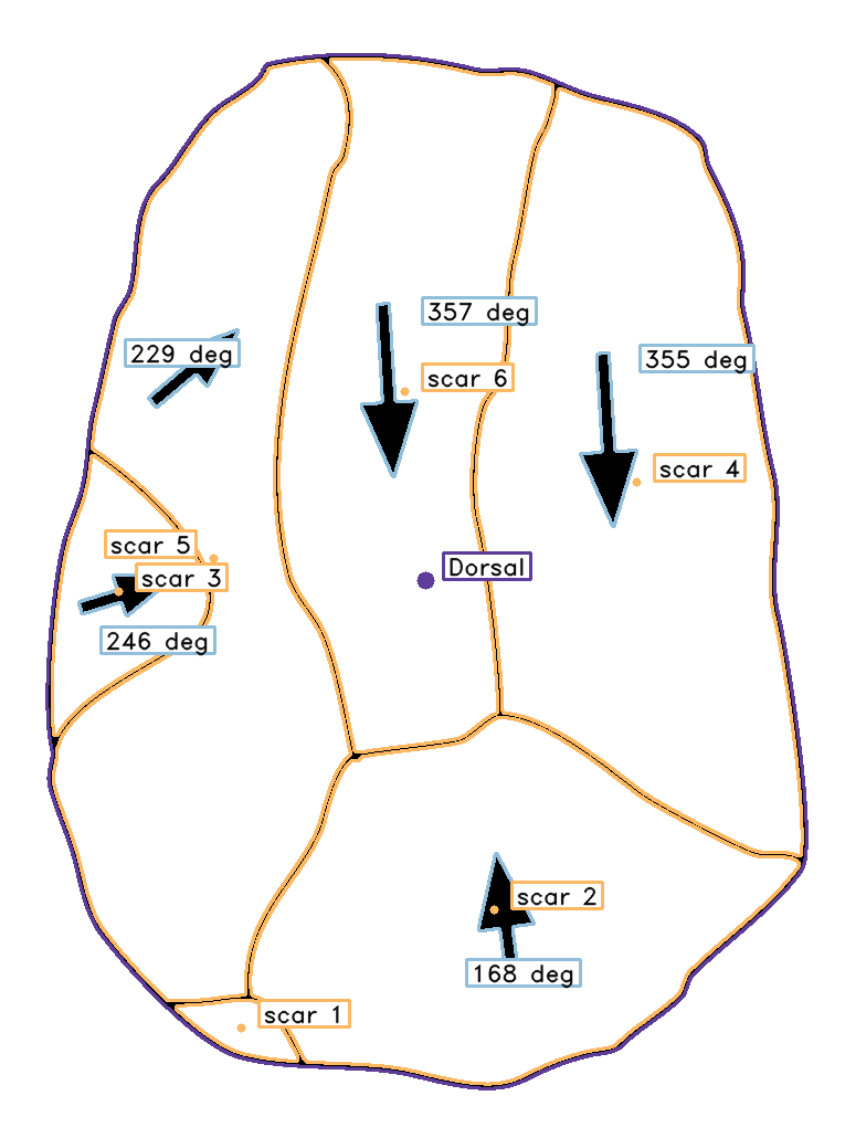
Surface classification and scar detection overlaid on the source image.

Voronoi Diagrams — {image_stem}_voronoi.png

A Voronoi tessellation of dorsal scar centroids with the convex hull outlined.

• One cell per centroid, clipped to the dorsal surface
• Axes in millimetres when scale calibration succeeded, pixels otherwise
• Convex hull drawn around all centroids

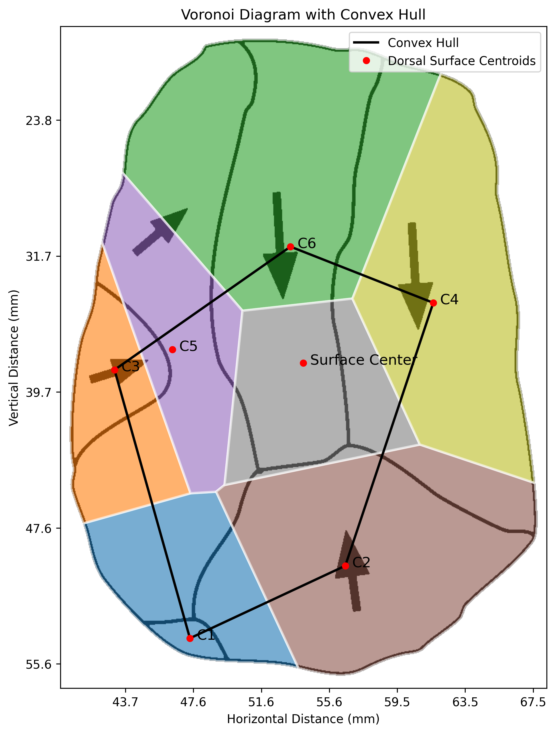
Voronoi tessellation showing spatial distribution of scar centroids.

Per-Lithic JSON Output (Optional)

When you pass --export_json, PyLithics writes one JSON file per lithic to processed/json/{image_stem}.json in addition to the CSV. The CSV is unchanged.

The JSON nests metrics by surface and feature, with calibration metadata at the top level:

{
  "schema_version": 1,
  "image_id": "awbari.png",
  "calibration": {
    "method": "scale_bar",
    "pixels_per_mm": 25.2,
    "scale_confidence": 1.0
  },
  "surfaces": [
    {
      "surface_type": "Dorsal",
      "surface_feature": "Dorsal",
      "centroid_x": 1361.76,
      "centroid_y": 957.21,
      "technical_width": 683.0,
      "technical_length": 936.0,
      "total_area": 525089.0,
      "scar_count": 6,
      "voronoi": {
        "num_cells": 7,
        "cell_area": 48384.82,
        "convex_hull_width": 468.98,
        "convex_hull_height": 576.02,
        "convex_hull_area": 165101.47
      },
      "symmetry": {
        "top_area": 257182.0,
        "bottom_area": 269162.0,
        "vertical_symmetry": 0.98,
        "horizontal_symmetry": 1.0
      },
      "lateral_convexity": null,
      "features": [
        {
          "surface_feature": "scar 1",
          "centroid_x": 1194.91,
          "centroid_y": 1362.25,
          "max_width": 33.38,
          "max_length": 120.02,
          "total_area": 3534.5,
          "voronoi_cell_area": 39808.67,
          "scar_complexity": 2,
          "is_cortex": false,
          "has_arrow": false
        }
      ]
    }
  ]
}

Schema rules

• One JSON file per lithic, written to processed/json/.
• schema_version is currently 1 and bumps on incompatible schema changes.
• null for absent values — every JSON file has the same fixed key set, so pd.json_normalize and R jsonlite::fromJSON produce rectangular dataframes with no surprise missing columns.
• Voronoi and symmetry blocks are nested under the Dorsal surface only; they are null on Ventral, Platform, and Lateral surfaces.
• lateral_convexity is a number on Lateral surfaces and null on the rest.
• Cortex children sit alongside scars in the Dorsal surface's features array, distinguished by is_cortex: true.
• Booleans (is_cortex, has_arrow) are JSON booleans, never strings.

Loading the JSON

import json, pandas as pd

with open("pylithics/data/processed/json/awbari.json") as f:
    doc = json.load(f)

# Flatten the dorsal features into a dataframe
dorsal = next(s for s in doc["surfaces"] if s["surface_type"] == "Dorsal")
features_df = pd.json_normalize(dorsal["features"])

library(jsonlite)

doc <- fromJSON("pylithics/data/processed/json/awbari.json",
                simplifyDataFrame = TRUE)

# Dorsal features as a data frame
dorsal <- doc$surfaces[doc$surfaces$surface_type == "Dorsal", ]
dorsal$features[[1]]

Processing Log: pylithics.log

The log captures the full per-step trace of every image the pipeline touches, regardless of how quiet you keep the console. Each run truncates the previous log by default so the file always reflects only the most recent invocation; if you need a history, copy the file off between runs or set a different log_file in config.yaml.

Verbosity model:

• File handler: always at DEBUG — every preprocessing step, every contour, every arrow assignment, every cortex variance reading.
• Console handler: INFO by default — startup metadata, one summary line per image, and the end-of-batch summary. Use --verbose (or -v) to mirror the file's DEBUG trace on screen.
• Third-party libraries (PIL, matplotlib, fontTools, asyncio) are pinned to WARNING. Their chatty internals never appear in your log.

Useful entries to grep for:

• Output directory: — where the run wrote its results
• <image_id> · <px/mm> — per-image summary at INFO (e.g. awbari.png · 25.20 px/mm)
• pixels (no scale provided) — image was processed in pixel-only mode by design
• pixels (scale detection failed — see log) — scale was provided but detection failed; a corresponding [WARNING] Scale image not found: or Scale bar detection returned no match line precedes it
• images processed without errors. / images processed successfully. — the end-of-batch summary line
• [WARNING] / [ERROR] — anything that surfaced above the default console level

A typical successful run looks like this:

2026-06-19 10:33:15 [INFO] Config: default
2026-06-19 10:33:15 [INFO] Data directory: pylithics/data
2026-06-19 10:33:15 [INFO] Metadata file: pylithics/data/meta_data.csv
2026-06-19 10:33:15 [INFO] Input validation passed
2026-06-19 10:33:15 [INFO] Output directory: pylithics/data/processed
2026-06-19 10:33:15 [DEBUG] Starting batch processing of 5 images
2026-06-19 10:33:15 [DEBUG] Processing image: awbari.png
... (per-step DEBUG trace for awbari) ...
2026-06-19 10:33:22 [INFO] awbari.png · 25.20 px/mm
2026-06-19 10:33:22 [DEBUG] Processing image: rub_al_khali.png
... etc. ...
2026-06-19 10:34:12 [INFO] qesem_cave.png · 25.20 px/mm
2026-06-19 10:34:12 [INFO] 5/5 images processed without errors.

If any image fails the pipeline raises, the summary becomes <N_succeeded>/<TOTAL> images processed successfully. and a [WARNING] Failed images: … line lists the offenders.

Validation Checklist

After each run, verify:

1. processed_metrics.csv exists and contains one row per image_id × surface_feature combination you expected
2. Each _labeled.png looks right — surface classification matches the artifact, no obvious mis-detected scars
3. Each Dorsal parent row has a Voronoi diagram if it has scars
4. calibration_method is scale_bar for images you provided scales for, and not silently pixels
5. Spot-check measurements: a typical flake should land in a sensible range (10–200 mm long, 100–15,000 mm² area)

Working with Output Data

R

data <- read.csv("pylithics/data/processed/processed_metrics.csv")

# Surface counts
table(data$surface_type, data$surface_feature)

# Length × width on dorsal surfaces
dorsal <- subset(data, surface_feature == "Dorsal")
plot(dorsal$technical_length, dorsal$technical_width,
     xlab = "Length (mm)", ylab = "Width (mm)",
     col = as.factor(dorsal$image_id))

Python

import pandas as pd
import matplotlib.pyplot as plt

df = pd.read_csv("pylithics/data/processed/processed_metrics.csv")

# Parent surfaces only
surfaces = df[df["surface_type"] == df["surface_feature"]]

plt.figure(figsize=(8, 6))
plt.scatter(surfaces["technical_length"], surfaces["technical_width"])
plt.xlabel("Length (mm)")
plt.ylabel("Width (mm)")
plt.title("Surface dimensions")
plt.show()

Next Steps

• Glossary — full reference for every column above