MLJ Cheatsheet

Starting an interactive MLJ session

julia> using MLJ
julia> MLJ_VERSION # version of MLJ for this cheatsheetv"0.20.2"

Model search and code loading

info("PCA") retrieves registry metadata for the model called "PCA"

info("RidgeRegressor", pkg="MultivariateStats") retrieves metadata for "RidgeRegresssor", which is provided by multiple packages

doc("DecisionTreeClassifier", pkg="DecisionTree") retrieves the model document string for the classifier, without loading model code

models() lists metadata of every registered model.

models("Tree") lists models with "Tree" in the model or package name.

models(x -> x.is_supervised && x.is_pure_julia) lists all supervised models written in pure julia.

models(matching(X)) lists all unsupervised models compatible with input X.

models(matching(X, y)) lists all supervised models compatible with input/target X/y.

With additional conditions:

models() do model
    matching(model, X, y) &&
    model.prediction_type == :probabilistic &&
        model.is_pure_julia
end

Tree = @load DecisionTreeClassifier pkg=DecisionTree imports "DecisionTreeClassifier" type and binds it to Tree tree = Tree() to instantiate a Tree.

tree2 = Tree(max_depth=2) instantiates a tree with different hyperparameter

Ridge = @load RidgeRegressor pkg=MultivariateStats imports a type for a model provided by multiple packages

For interactive loading instead, use @iload

Scitypes and coercion

scitype(x) is the scientific type of x. For example scitype(2.4) == Continuous

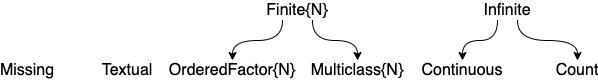
type	scitype
`AbstractFloat`	`Continuous`
`Integer`	`Count`
`CategoricalValue` and `CategoricalString`	`Multiclass` or `OrderedFactor`
`AbstractString`	`Textual`

Figure and Table for common scalar scitypes

Use schema(X) to get the column scitypes of a table X

coerce(y, Multiclass) attempts coercion of all elements of y into scitype Multiclass

coerce(X, :x1 => Continuous, :x2 => OrderedFactor) to coerce columns :x1 and :x2 of table X.

coerce(X, Count => Continuous) to coerce all columns with Count scitype to Continuous.

Ingesting data

Split the table channing into target y (the :Exit column) and features X (everything else), after a seeded row shuffling:

using RDatasets
channing = dataset("boot", "channing")
y, X =  unpack(channing, ==(:Exit); rng=123)

Same as above but exclude :Time column from X:

using RDatasets
channing = dataset("boot", "channing")
y, X =  unpack(channing,
               ==(:Exit),            # y is the :Exit column
               !=(:Time);            # X is the rest, except :Time
               rng=123)

Splitting row indices into train/validation/test, with seeded shuffling:

train, valid, test = partition(eachindex(y), 0.7, 0.2, rng=1234) for 70:20:10 ratio

For a stratified split:

train, test = partition(eachindex(y), 0.8, stratify=y)

Split a table or matrix X, instead of indices:

Xtrain, Xvalid, Xtest = partition(X, 0.5, 0.3, rng=123)

Getting data from OpenML:

table = OpenML.load(91)

Creating synthetic classification data:

X, y = make_blobs(100, 2) (also: make_moons, make_circles)

Creating synthetic regression data:

X, y = make_regression(100, 2)

Machine construction

Supervised case:

model = KNNRegressor(K=1) and mach = machine(model, X, y)

Unsupervised case:

model = OneHotEncoder() and mach = machine(model, X)

Fitting

fit!(mach, rows=1:100, verbosity=1, force=false) (defaults shown)

Prediction

Supervised case: predict(mach, Xnew) or predict(mach, rows=1:100)

Similarly, for probabilistic models: predict_mode, predict_mean and predict_median.

Unsupervised case: transform(mach, rows=1:100) or inverse_transform(mach, rows), etc.

Inspecting objects

@more gets detail on the last object in REPL

params(model) gets a nested-tuple of all hyperparameters, even nested ones

info(ConstantRegressor()), info("PCA"), info("RidgeRegressor", pkg="MultivariateStats") gets all properties (aka traits) of registered models

info(rms) gets all properties of a performance measure

schema(X) get column names, types and scitypes, and nrows, of a table X

scitype(X) gets the scientific type of X

fitted_params(mach) gets learned parameters of the fitted machine

report(mach) gets other training results (e.g. feature rankings)

Saving and retrieving machines using Julia serializer

MLJ.save("trained_for_five_days.jls", mach) to save machine mach (without data)

predict_only_mach = machine("trained_for_five_days.jlso") to deserialize.

Performance estimation

evaluate(model, X, y, resampling=CV(), measure=rms, operation=predict, weights=..., verbosity=1)

evaluate!(mach, resampling=Holdout(), measure=[rms, mav], operation=predict, weights=..., verbosity=1)

evaluate!(mach, resampling=[(fold1, fold2), (fold2, fold1)], measure=rms)

Resampling strategies (`resampling=...`)

Holdout(fraction_train=0.7, rng=1234) for simple holdout

CV(nfolds=6, rng=1234) for cross-validation

StratifiedCV(nfolds=6, rng=1234) for stratified cross-validation

TimeSeriesSV(nfolds=4) for time-series cross-validation

or a list of pairs of row indices:

[(train1, eval1), (train2, eval2), ... (traink, evalk)]

Tuning

Tuning model wrapper

tuned_model = TunedModel(model=…, tuning=RandomSearch(), resampling=Holdout(), measure=…, operation=predict, range=…)

Ranges for tuning (`range=...`)

If r = range(KNNRegressor(), :K, lower=1, upper = 20, scale=:log)

then Grid() search uses iterator(r, 6) == [1, 2, 3, 6, 11, 20].

lower=-Inf and upper=Inf are allowed.

Non-numeric ranges: r = range(model, :parameter, values=…)

Nested ranges: Use dot syntax, as in r = range(EnsembleModel(atom=tree), :(atom.max_depth), ...)

Can specify multiple ranges, as in range=[r1, r2, r3]. For more range options do ?Grid or ?RandomSearch

Tuning strategies

RandomSearch(rng=1234) for basic random search

Grid(resolution=10) or Grid(goal=50) for basic grid search

Also available: LatinHyperCube, Explicit (built-in), MLJTreeParzenTuning, ParticleSwarm, AdaptiveParticleSwarm (3rd-party packages)

Learning curves

For generating a plot of performance against parameter specified by range:

curve = learning_curve(mach, resolution=30, resampling=Holdout(), measure=…, operation=predict, range=…, n=1)

curve = learning_curve(model, X, y, resolution=30, resampling=Holdout(), measure=…, operation=predict, range=…, n=1)

If using Plots.jl:

plot(curve.parameter_values, curve.measurements, xlab=curve.parameter_name, xscale=curve.parameter_scale)

Controlling iterative models

Requires: using MLJIteration

iterated_model = IteratedModel(model=…, resampling=Holdout(), measure=…, controls=…, retrain=false)

Controls

Increment training: Step(n=1)

Stopping: TimeLimit(t=0.5) (in hours), NumberLimit(n=100), NumberSinceBest(n=6), NotANumber(), Threshold(value=0.0), GL(alpha=2.0), PQ(alpha=0.75, k=5), Patience(n=5)

Logging: Info(f=identity), Warn(f=""), Error(predicate, f="")

Callbacks: Callback(f=mach->nothing), WithNumberDo(f=n->@info(n)), WithIterationsDo(f=i->@info("num iterations: $i")), WithLossDo(f=x->@info("loss: $x")), WithTrainingLossesDo(f=v->@info(v))

Snapshots: Save(filename="machine.jlso")

Wraps: MLJIteration.skip(control, predicate=1), IterationControl.with_state_do(control)

Performance measures (metrics)

Do measures() to get full list.

info(rms) to list properties (aka traits) of the rms measure

Transformers

Built-ins include: Standardizer, OneHotEncoder, UnivariateBoxCoxTransformer, FeatureSelector, FillImputer, UnivariateDiscretizer, ContinuousEncoder, UnivariateTimeTypeToContinuous

Externals include: PCA (in MultivariateStats), KMeans, KMedoids (in Clustering).

models(m -> !m.is_supervised) to get full list

pipe = Standardizer |> OneHotEncoder

Concatenation:

pipe1 |> pipe2 or model |> pipe or pipe |> model, etc

Define a supervised learning network:

Xs = source(X) ys = source(y)

... define further nodal machines and nodes ...

yhat = predict(knn_machine, W, ys) (final node)

Exporting a learning network as a stand-alone model:

Supervised, with final node yhat returning point predictions:

@from_network machine(Deterministic(), Xs, ys; predict=yhat) begin
    mutable struct Composite
	    reducer=network_pca
		regressor=network_knn
    end

Here network_pca and network_knn are models appearing in the learning network.

Supervised, with yhat final node returning probabilistic predictions:

@from_network machine(Probabilistic(), Xs, ys; predict=yhat) begin
    mutable struct Composite
        reducer=network_pca
        classifier=network_tree
    end

Unsupervised, with final node Xout:

@from_network machine(Unsupervised(), Xs; transform=Xout) begin
    mutable struct Composite
	    reducer1=network_pca
		reducer2=clusterer
    end
end

UnivariateTimeTypeToContinuous