1 Identifying Runs for bias correction
Ruth C E Bowyer 2023-06-13
rm(list=ls())

library(tidyverse)
library(ggplot2)
library(RColorBrewer)
1.1 0. About
Script to identify the mean, 2nd highest and 2nd lowers daily tasmax per UKCP18 CPM run.
These runs will be the focus of initial bias correction focus
1.2 1. Load Data
Data is tasmax runs converted to dataframe using sript ‘ConvertingAllCPMdataTOdf.R’, with files later renamed.Then daily means for historical periods and future periods were calculated using ‘calc.mean.sd.daily.R’ and summaries saved as .csv
In retrospect the conversion to df might not have been necessary/the most resource efficient, see comment here:https://tmieno2.github.io/R-as-GIS-for-Economists/turning-a-raster-object-into-a-data-frame.html – this was tested and using terra::global to calculate the raster-wide mean was less efficient
Update 13.05.23 - Adding in infill data, mean to be calculated over the whole time period
As of June 2023, the tasmax-as-dataframe and tasmax daily means and the df data is located in vmfileshare/Interim/tasmax_dfs/
There is an error in the naming convention - Y00_Y20 should be Y01 to reflect the infill data time period (although this does cover a breif period of 2000) - to be updated in future
Runs <- c("01", "04", "05", "06", "07", "08", "09", "10", "11", "12", "13", "15")

files <- list.files("/Users/rbowyer/Library/CloudStorage/OneDrive-TheAlanTuringInstitute/tempdata/")

files <- files[grepl(".csv", files)]
fp <- paste0("/Users/rbowyer/Library/CloudStorage/OneDrive-TheAlanTuringInstitute/tempdata/", files)
# Creating objects for names and filepath for each of the timer periods, for easy loading
names <- gsub("df.avs_|.csv|df.", "", files)
i <- c("hist", "Y00_Y20","Y21_Y40", "Y41_Y60", "Y61_Y80")
namesL <- lapply(i, function(i){
n <- names[grepl(i, names)]
})
names(namesL) <- paste0("names_",i)
list2env(namesL, .GlobalEnv)## <environment: R_GlobalEnv>dfL <- lapply(i, function(i){
fp <- fp[grepl(i, fp)]
dfs <- lapply(fp, read.csv)
n <- namesL[[paste0("names_",i)]]
names(dfs) <- n
return(dfs)
})
names(dfL) <- paste0("dfs_", i)
list2env(dfL, .GlobalEnv)## <environment: R_GlobalEnv>1.3 2. Comparing Runs
1.3.1 2a. Historical figures
Y <- rep(c(1981:2000), each=360)

dfs_hist <- lapply(names_hist, function(i){
  df <- dfs_hist[[i]]
  names(df) <- c("day", "mean", "sd")
  df$model <- i
  df$dn <- 1:nrow(df)
  df$Y <- Y
  return(df)
})

#Create a single df in long form of Runs for the historical period
historical_means <- dfs_hist %>% reduce(rbind)
1.3.2 Time series - daily
ggplot(historical_means) +
    geom_line(aes(x=dn, y=mean, group=model, colour=model)) +

    theme_bw() + xlab("Day (Historical 1980 - 2000)") +
    ylab("Daily mean max temp (tasmax) oC") +

   scale_colour_brewer(palette = "Paired", name = "") +
    theme(axis.text.x=element_blank(),
        axis.ticks.x=element_blank(),
        legend.position = "none") +
  facet_wrap(.~ model, ncol=3)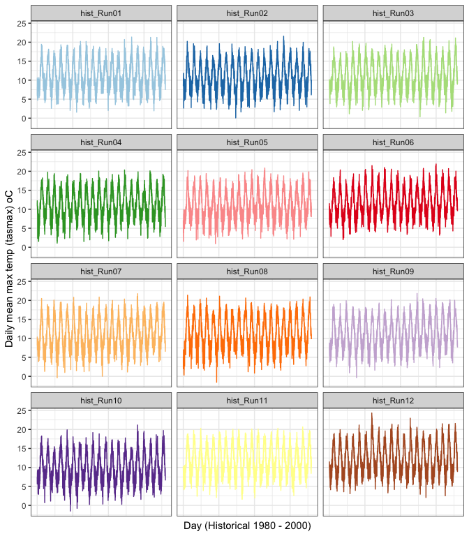
1.3.3 boxplot - mean historical
#Create a pallete specific to the runs so when reordered maintain the same colours
historical_means$model <- as.factor(historical_means$model)
c <- brewer.pal(12, "Paired")
my_colours <- setNames(c, levels(historical_means$model))
historical_means %>%
mutate(model = fct_reorder(model, mean, .fun='median')) %>%
ggplot(aes(x=reorder(model, mean), y=mean, fill=model)) +
geom_boxplot() + theme_bw() +
ylab("Mean daily max temp (tasmax) oC") + xlab("model") +
scale_fill_manual(values = my_colours) +
theme(axis.text.x=element_blank(),
axis.ticks.x=element_blank())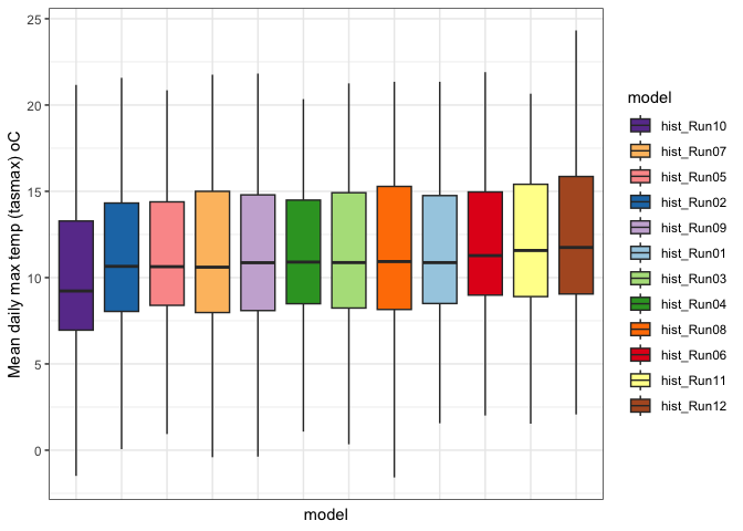
1.3.4 qqplot - daily means
ggplot(historical_means, aes(sample=mean, colour=factor(model))) +
  stat_qq() +
  stat_qq_line()+
  theme_bw()+
  scale_color_manual(values = my_colours) +
  facet_wrap(.~model, ncol=3)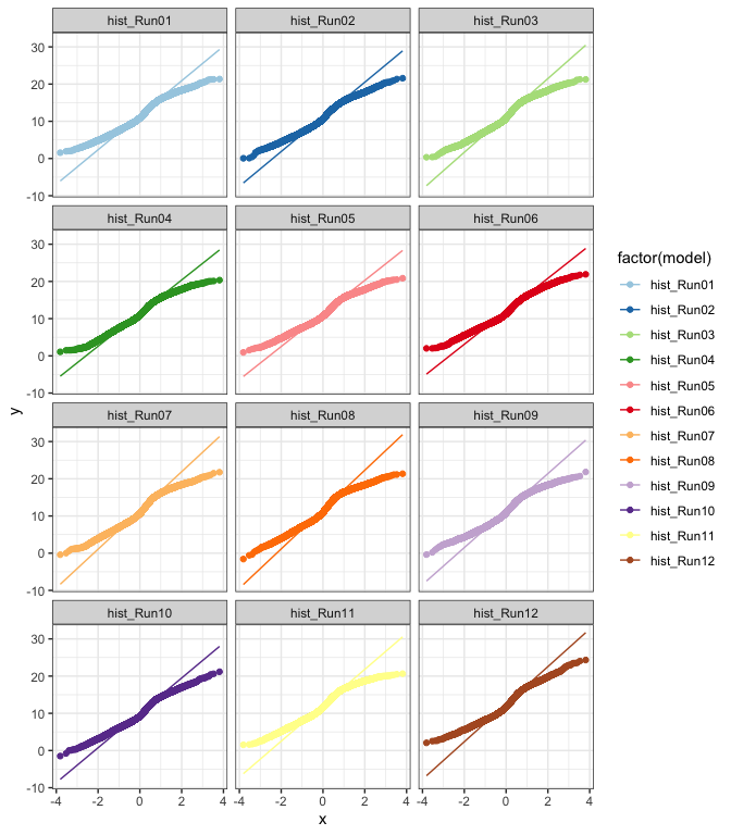
1.3.5 Time series - annual mean
#Aggregating to year for annual average

historical_means$Yf <- as.factor(historical_means$Y)

historical_means_y <- historical_means %>%
  group_by(Yf, model) %>%
dplyr::summarise(mean.annual=mean(mean, na.rm=T), sd.annual=sd(mean, na.rm = T))ggplot(historical_means_y) +
geom_line(aes(x = as.numeric(Yf), y=mean.annual,
color=model)) +
theme_bw() + xlab("Year (Historical 1980 - 2000)") +
ylab("Annual mean of mean daily max temp (tasmax) oC") +
scale_fill_brewer(palette = "Paired", name = "") +
scale_colour_brewer(palette = "Paired", name = "") +
theme(axis.text.x=element_blank(),
axis.ticks.x=element_blank())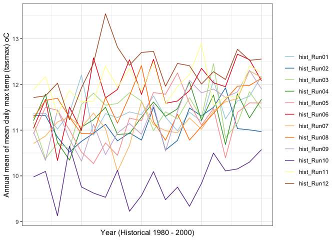
# Plotting with SDs in geom_ribbon to see if anything wildely different
ggplot(historical_means_y) +
    geom_ribbon(aes(as.numeric(Yf), y=mean.annual,
                               ymin = mean.annual - sd.annual,
                              ymax= mean.annual + sd.annual,
                    fill=model),  alpha=0.4) +
    geom_line(aes(x = as.numeric(Yf), y=mean.annual,
              color=model)) +
    theme_bw() + xlab("Year (Historical 1980 - 2000)") +
    ylab("Annual mean of mean daily max temp (tasmax) oC") +
  scale_fill_brewer(palette = "Paired", name = "") +
   scale_colour_brewer(palette = "Paired", name = "") +
    theme(axis.text.x=element_blank(),
        axis.ticks.x=element_blank()) + facet_wrap(.~model, ncol=3)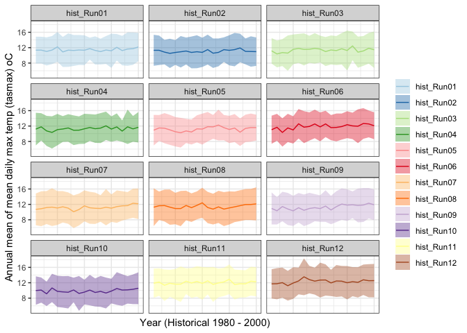
1.3.6 boxplot - annual mean historical
historical_means_y %>%
  mutate(model = fct_reorder(model, mean.annual, .fun='median')) %>%
    ggplot(aes(x=reorder(model, mean.annual), y=mean.annual, fill=model)) +
    geom_boxplot() + theme_bw() +
    ylab("Annual max daily max temp oC") + xlab("model") +
   scale_fill_manual(values = my_colours) +
    theme(axis.text.x=element_blank(),
        axis.ticks.x=element_blank())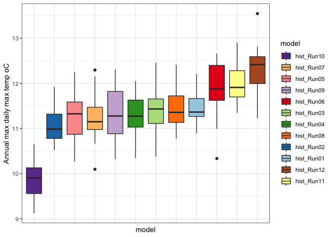
1.3.7 qqplot - annual means
ggplot(historical_means_y, aes(sample=mean.annual, colour=factor(model))) +
  stat_qq() +
  stat_qq_line()+
  theme_bw()+
  scale_color_manual(values = my_colours) +
  facet_wrap(.~model, ncol=3)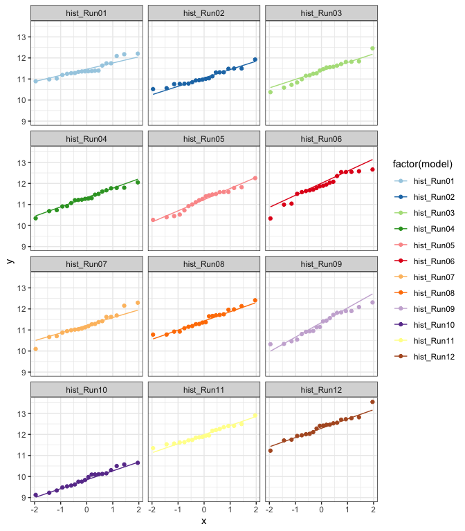
1.3.8 Time series - annual max
historical_max_y <- historical_means %>%
  group_by(Yf, model) %>%
dplyr::summarise(max=max(mean, na.rm=T))ggplot(historical_max_y) +
geom_line(aes(x = as.numeric(Yf), y=max,
color=model)) +
theme_bw() + xlab("Year (Historical 1980 - 2000)") +
ylab("Annual max of mean daily max temp (tasmax) oC") +
scale_fill_brewer(palette = "Paired", name = "") +
scale_colour_brewer(palette = "Paired", name = "") +
theme(axis.text.x=element_blank(),
axis.ticks.x=element_blank())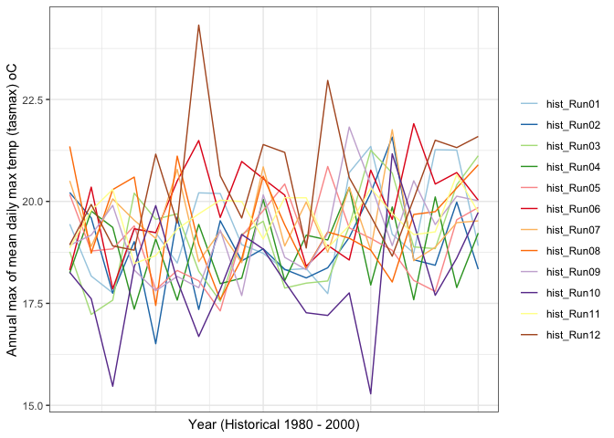
1.3.9 boxplot - annual max
historical_max_y %>%
  mutate(model = fct_reorder(model, max, .fun='median')) %>%
    ggplot(aes(x=reorder(model, max), y=max, fill=model)) +
    geom_boxplot() + theme_bw() +
    ylab("Annual max of mean daily max temp (tasmax) oC") + xlab("model") +
   scale_fill_manual(values = my_colours) +
    theme(axis.text.x=element_blank(),
        axis.ticks.x=element_blank())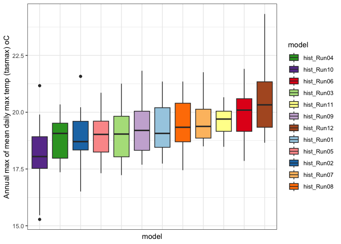
The daily max is quite different than the means - something to bear in mind but interesting to think about - eg Run 4 here has the 2nd lowest spread of max max temp, but is selected above based on means
1.3.10 ANOVA
Daily means:
#-1 removes the intercept to compare coefficients of all Runs
av1 <- aov(mean ~ model - 1, historical_means)
av1$coefficients[order(av1$coefficients)]
## modelhist_Run10 modelhist_Run02 modelhist_Run05 modelhist_Run07 modelhist_Run09
## 9.89052 11.06863 11.21424 11.22048 11.27647
## modelhist_Run04 modelhist_Run03 modelhist_Run08 modelhist_Run01 modelhist_Run06
## 11.29057 11.35848 11.45257 11.45414 11.86451
## modelhist_Run11 modelhist_Run12
## 11.99148 12.31870Annual means:
av2 <- aov(mean.annual ~ model - 1, historical_means_y)
av2$coefficients[order(av2$coefficients)]
## modelhist_Run10 modelhist_Run02 modelhist_Run05 modelhist_Run07 modelhist_Run09
## 9.89052 11.06863 11.21424 11.22048 11.27647
## modelhist_Run04 modelhist_Run03 modelhist_Run08 modelhist_Run01 modelhist_Run06
## 11.29057 11.35848 11.45257 11.45414 11.86451
## modelhist_Run11 modelhist_Run12
## 11.99148 12.31870Max of means:
av3 <- aov(max ~ model - 1, historical_max_y)
av3$coefficients[order(av3$coefficients)]
## modelhist_Run10 modelhist_Run04 modelhist_Run02 modelhist_Run05 modelhist_Run03
## 18.12329 18.81126 18.90054 19.01801 19.10454
## modelhist_Run09 modelhist_Run01 modelhist_Run08 modelhist_Run07 modelhist_Run11
## 19.23705 19.31541 19.44439 19.54981 19.57548
## modelhist_Run06 modelhist_Run12
## 19.88375 20.47650Max vals are different but based on means then selection would be Run 02 (2nd lowest), Run 04 & Run 03, and Run 11 (2nd lowest)
1.3.11 2b. Y2020 - Y2040
Y <- rep(c(2021:2040), each=360)


dfs_Y21_Y40 <- lapply(names_Y21_Y40, function(i){
  df <- dfs_Y21_Y40[[i]]
  names(df) <- c("day", "mean", "sd")
  df$model <- i
  df$dn <- 1:nrow(df)
  df$Y <- Y
  return(df)
})

#Create a single df in long form of Runs for the Y21_Y40 period
Y21_Y40_means <- dfs_Y21_Y40 %>% reduce(rbind)
1.3.12 Time series - daily
ggplot(Y21_Y40_means) +
    geom_line(aes(x=dn, y=mean, group=model, colour=model)) +
  # Removing sd ribbon for ease of viewing
  #geom_ribbon(aes(x =dn, ymin = mean - sd, ymax= mean + sd), alpha=0.4) +
    theme_bw() + xlab("Daily (1980 - 2000)") +
    ylab("Daily mean max temp (tasmax) oC") +
  #scale_fill_brewer(palette = "Paired", name = "") +
   scale_colour_brewer(palette = "Paired", name = "") +
    theme(axis.text.x=element_blank(),
        axis.ticks.x=element_blank(),
        legend.position = "none") +
  facet_wrap(.~ model, ncol=3) + guides(fill = FALSE)
## Warning: The `<scale>` argument of `guides()` cannot be `FALSE`. Use "none" instead as
## of ggplot2 3.3.4.
## This warning is displayed once every 8 hours.
## Call `lifecycle::last_lifecycle_warnings()` to see where this warning was
## generated.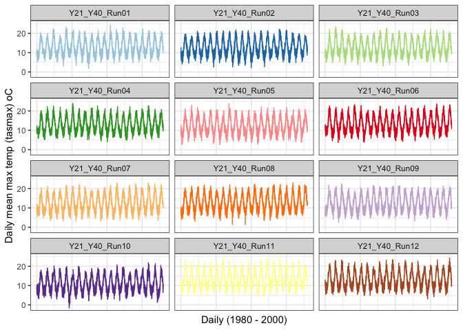
1.3.13 boxplot - mean Y21_Y40
#Create a pallete specific to the runs so when reordered maintain the same colours
Y21_Y40_means$model <- as.factor(Y21_Y40_means$model)
c <- brewer.pal(12, "Paired")
my_colours <- setNames(c, levels(Y21_Y40_means$model))
Y21_Y40_means %>%
mutate(model = fct_reorder(model, mean, .fun='median')) %>%
ggplot(aes(x=reorder(model, mean), y=mean, fill=model)) +
geom_boxplot() + theme_bw() +
ylab("Mean daily max temp (tasmax) oC") + xlab("model") +
scale_fill_manual(values = my_colours) +
theme(axis.text.x=element_blank(),
axis.ticks.x=element_blank())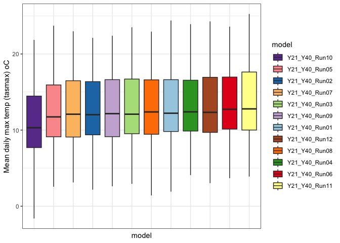
1.3.14 qqplot - daily means
ggplot(Y21_Y40_means, aes(sample=mean, colour=factor(model))) +
  stat_qq() +
  stat_qq_line()+
  theme_bw()+
  scale_color_manual(values = my_colours) +
  facet_wrap(.~model, ncol=3)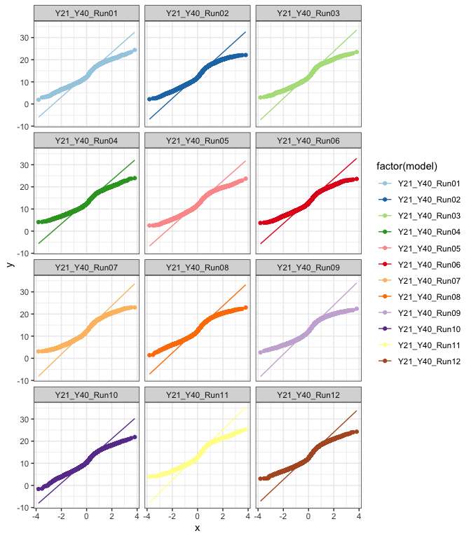
1.3.15 Time series - annual mean
#Aggregating to year for annual average

Y21_Y40_means$Yf <- as.factor(Y21_Y40_means$Y)

Y21_Y40_means_y <- Y21_Y40_means %>%
  group_by(Yf, model) %>%
dplyr::summarise(mean.annual=mean(mean, na.rm=T), sd.annual=sd(mean, na.rm = T))ggplot(Y21_Y40_means_y) +
geom_line(aes(x = as.numeric(Yf), y=mean.annual,
color=model)) +
theme_bw() + xlab("Year (2021 - 2040)") +
ylab("Annual mean of mean daily max temp (tasmax) oC") +
scale_fill_brewer(palette = "Paired", name = "") +
scale_colour_brewer(palette = "Paired", name = "") +
theme(axis.text.x=element_blank(),
axis.ticks.x=element_blank())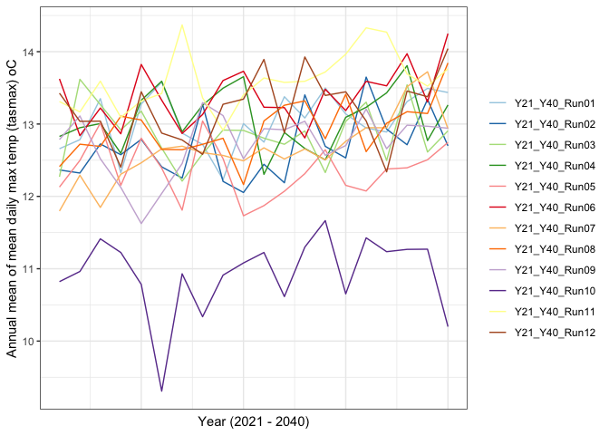
# Plotting with SDs in geom_ribbon to see if anything wildely different
ggplot(Y21_Y40_means_y) +
    geom_ribbon(aes(as.numeric(Yf), y=mean.annual,
                               ymin = mean.annual - sd.annual,
                              ymax= mean.annual + sd.annual,
                    fill=model),  alpha=0.4) +
    geom_line(aes(x = as.numeric(Yf), y=mean.annual,
              color=model)) +
    theme_bw() + xlab("Year (2021 - 2040)") +
    ylab("Annual mean of mean daily max temp (tasmax) oC") +
  scale_fill_brewer(palette = "Paired", name = "") +
   scale_colour_brewer(palette = "Paired", name = "") +
    theme(axis.text.x=element_blank(),
        axis.ticks.x=element_blank()) + facet_wrap(.~model, ncol=3)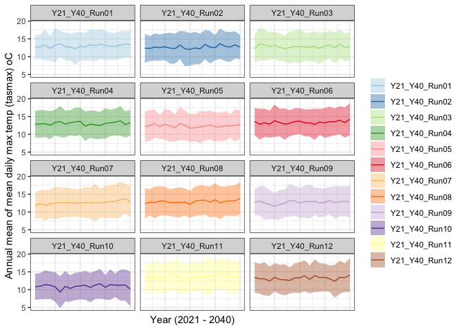
1.3.16 boxplot - annual mean 2021 - 2040
Y21_Y40_means_y %>%
  mutate(model = fct_reorder(model, mean.annual, .fun='median')) %>%
    ggplot(aes(x=reorder(model, mean.annual), y=mean.annual, fill=model)) +
    geom_boxplot() + theme_bw() +
    ylab("Annual max daily max temp oC") + xlab("model") +
   scale_fill_manual(values = my_colours) +
    theme(axis.text.x=element_blank(),
        axis.ticks.x=element_blank())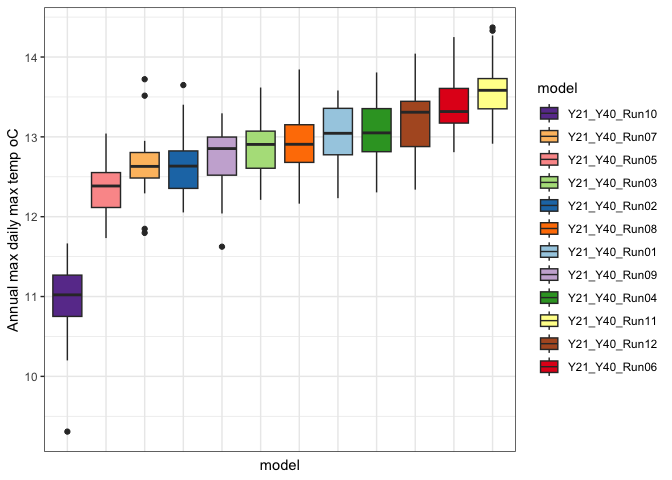
1.3.17 qqplot - annual means
ggplot(Y21_Y40_means_y, aes(sample=mean.annual, colour=factor(model))) +
  stat_qq() +
  stat_qq_line()+
  theme_bw()+
  scale_color_manual(values = my_colours) +
  facet_wrap(.~model, ncol=3)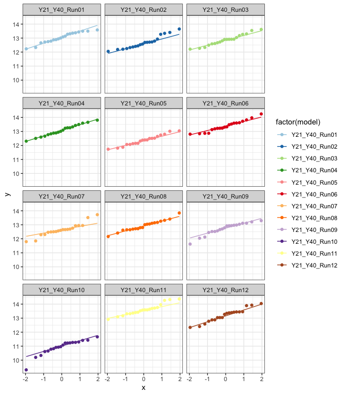
1.3.18 Time series - annual max
Y21_Y40_max_y <- Y21_Y40_means %>%
  group_by(Yf, model) %>%
dplyr::summarise(max=max(mean, na.rm=T))ggplot(Y21_Y40_max_y) +
geom_line(aes(x = as.numeric(Yf), y=max,
color=model)) +
theme_bw() + xlab("Year (2021 - 2040)") +
ylab("Annual max of mean daily max temp (tasmax) oC") +
scale_fill_brewer(palette = "Paired", name = "") +
scale_colour_brewer(palette = "Paired", name = "") +
theme(axis.text.x=element_blank(),
axis.ticks.x=element_blank())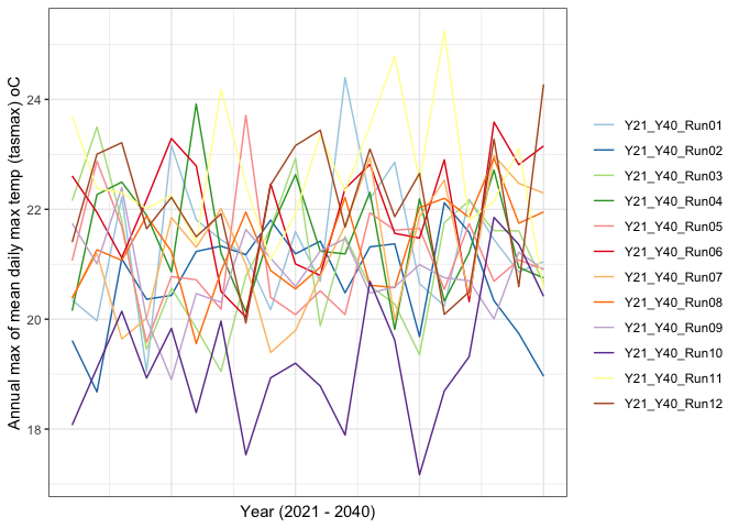
1.3.19 boxplot - annual max
Y21_Y40_max_y %>%
  mutate(model = fct_reorder(model, max, .fun='median')) %>%
    ggplot(aes(x=reorder(model, max), y=max, fill=model)) +
    geom_boxplot() + theme_bw() +
    ylab("Annual max of mean daily max temp (tasmax) oC") + xlab("model") +
   scale_fill_manual(values = my_colours) +
    theme(axis.text.x=element_blank(),
        axis.ticks.x=element_blank())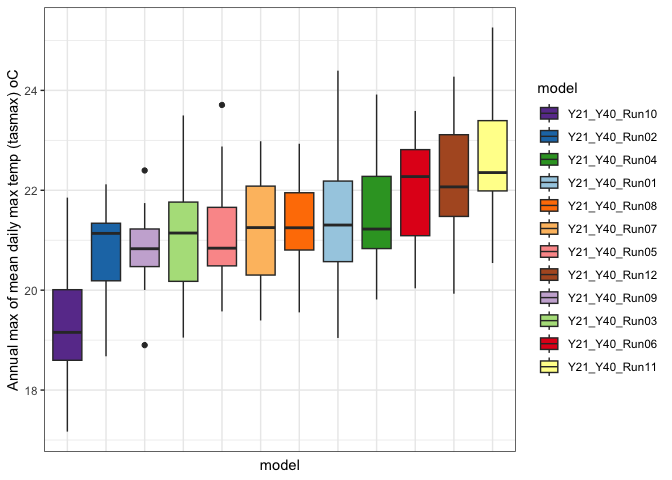
1.3.20 ANOVA
Daily means:
#-1 removes the intercept to compare coefficients of all Runs
av1 <- aov(mean ~ model - 1, Y21_Y40_means)
av1$coefficients[order(av1$coefficients)]
## modelY21_Y40_Run10 modelY21_Y40_Run05 modelY21_Y40_Run07 modelY21_Y40_Run02
## 10.93136 12.36223 12.64493 12.67791
## modelY21_Y40_Run09 modelY21_Y40_Run03 modelY21_Y40_Run08 modelY21_Y40_Run01
## 12.72584 12.85999 12.92934 13.03640
## modelY21_Y40_Run04 modelY21_Y40_Run12 modelY21_Y40_Run06 modelY21_Y40_Run11
## 13.07768 13.20011 13.38047 13.60076Annual means:
av2 <- aov(mean.annual ~ model - 1, Y21_Y40_means_y)
av2$coefficients[order(av2$coefficients)]
## modelY21_Y40_Run10 modelY21_Y40_Run05 modelY21_Y40_Run07 modelY21_Y40_Run02
## 10.93136 12.36223 12.64493 12.67791
## modelY21_Y40_Run09 modelY21_Y40_Run03 modelY21_Y40_Run08 modelY21_Y40_Run01
## 12.72584 12.85999 12.92934 13.03640
## modelY21_Y40_Run04 modelY21_Y40_Run12 modelY21_Y40_Run06 modelY21_Y40_Run11
## 13.07768 13.20011 13.38047 13.60076Max of means
av3 <- aov(max ~ model - 1, Y21_Y40_max_y)
av3$coefficients[order(av3$coefficients)]
## modelY21_Y40_Run10 modelY21_Y40_Run02 modelY21_Y40_Run09 modelY21_Y40_Run03
## 19.29044 20.69596 20.82538 21.05558
## modelY21_Y40_Run05 modelY21_Y40_Run07 modelY21_Y40_Run08 modelY21_Y40_Run01
## 21.09128 21.22942 21.33484 21.37443
## modelY21_Y40_Run04 modelY21_Y40_Run06 modelY21_Y40_Run12 modelY21_Y40_Run11
## 21.49363 21.98667 22.09476 22.65178Based on means then selection would be Run 02 (2nd lowest), Run 04 & Run 03, and Run 11 (2nd lowest)
Based on this period, the seelction would be: Run 05, Run 03, Run 08, Run 06 (so definetly Run 3 but others to be discussed)
1.3.21 2c. Y2061 - Y2080
Y <- rep(c(2061:2080), each=360)


dfs_Y61_Y80 <- lapply(names_Y61_Y80, function(i){
  df <- dfs_Y61_Y80[[i]]
  names(df) <- c("day", "mean", "sd")
  df$model <- i
  df$dn <- 1:nrow(df)
  df$Y <- Y
  return(df)
})

#Create a single df in long form of Runs for the Y61_Y80 period
Y61_Y80_means <- dfs_Y61_Y80 %>% reduce(rbind)
1.3.22 Time series - daily
ggplot(Y61_Y80_means) +
    geom_line(aes(x=dn, y=mean, group=model, colour=model)) +
  # Removing sd ribbon for ease of viewing
  #geom_ribbon(aes(x =dn, ymin = mean - sd, ymax= mean + sd), alpha=0.4) +
    theme_bw() + xlab("Day (2060 - 2080)") +
    ylab("Daily mean max temp (tasmax) oC") +
  #scale_fill_brewer(palette = "Paired", name = "") +
   scale_colour_brewer(palette = "Paired", name = "") +
    theme(axis.text.x=element_blank(),
        axis.ticks.x=element_blank(),
        legend.position = "none") +
  facet_wrap(.~ model, ncol=3) + guides(fill = FALSE)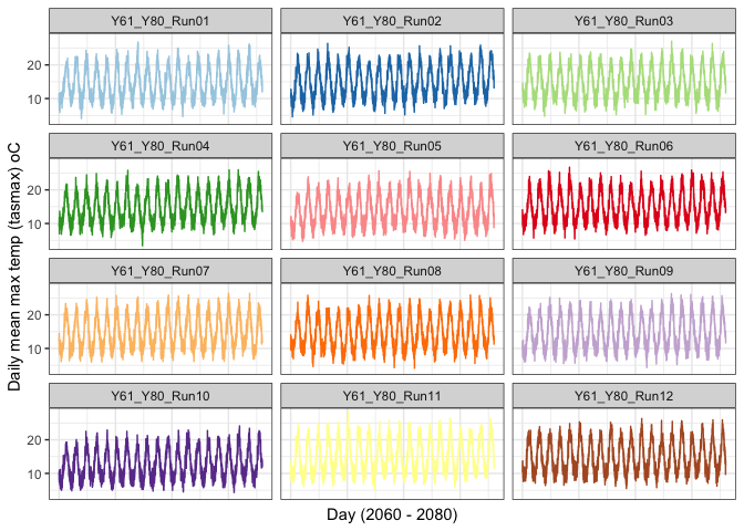
1.3.23 boxplot - mean Y61_Y80
#Create a pallete specific to the runs so when reordered maintain the same colours
Y61_Y80_means$model <- as.factor(Y61_Y80_means$model)
c <- brewer.pal(12, "Paired")
my_colours <- setNames(c, levels(Y61_Y80_means$model))
Y61_Y80_means %>%
mutate(model = fct_reorder(model, mean, .fun='median')) %>%
ggplot(aes(x=reorder(model, mean), y=mean, fill=model)) +
geom_boxplot() + theme_bw() +
ylab("Mean daily max temp (tasmax) oC") + xlab("model") +
scale_fill_manual(values = my_colours) +
theme(axis.text.x=element_blank(),
axis.ticks.x=element_blank())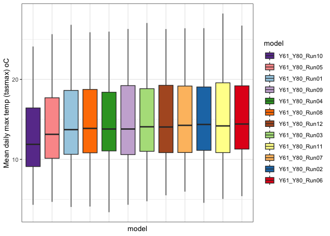
1.3.24 qqplot - daily means
ggplot(Y61_Y80_means, aes(sample=mean, colour=factor(model))) +
  stat_qq() +
  stat_qq_line()+
  theme_bw()+
  scale_color_manual(values = my_colours) +
  facet_wrap(.~model, ncol=3)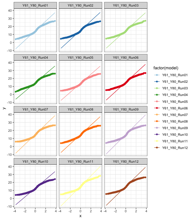
1.3.25 Time series - annual mean
#Aggregating to year for annual average

Y61_Y80_means$Yf <- as.factor(Y61_Y80_means$Y)

Y61_Y80_means_y <- Y61_Y80_means %>%
  group_by(Yf, model) %>%
dplyr::summarise(mean.annual=mean(mean, na.rm=T), sd.annual=sd(mean, na.rm = T))ggplot(Y61_Y80_means_y) +
geom_line(aes(x = as.numeric(Yf), y=mean.annual,
color=model)) +
theme_bw() + xlab("Year (2061 - 2080)") +
ylab("Annual mean of mean daily max temp (tasmax) oC") +
scale_fill_brewer(palette = "Paired", name = "") +
scale_colour_brewer(palette = "Paired", name = "") +
theme(axis.text.x=element_blank(),
axis.ticks.x=element_blank())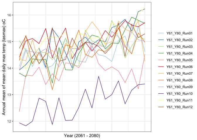
# Plotting with SDs in geom_ribbon to see if anything wildely different
ggplot(Y61_Y80_means_y) +
    geom_ribbon(aes(as.numeric(Yf), y=mean.annual,
                               ymin = mean.annual - sd.annual,
                              ymax= mean.annual + sd.annual,
                    fill=model),  alpha=0.4) +
    geom_line(aes(x = as.numeric(Yf), y=mean.annual,
              color=model)) +
    theme_bw() + xlab("Year (2061 - 2080)") +
    ylab("Annual mean of mean daily max temp (tasmax) oC") +
  scale_fill_brewer(palette = "Paired", name = "") +
   scale_colour_brewer(palette = "Paired", name = "") +
    theme(axis.text.x=element_blank(),
        axis.ticks.x=element_blank()) + facet_wrap(.~model, ncol=3)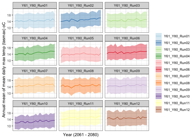
1.3.26 boxplot - annual mean Y61_Y80
Y61_Y80_means_y %>%
  mutate(model = fct_reorder(model, mean.annual, .fun='median')) %>%
    ggplot(aes(x=reorder(model, mean.annual), y=mean.annual, fill=model)) +
    geom_boxplot() + theme_bw() +
    ylab("Annual max daily max temp oC") + xlab("model") +
   scale_fill_manual(values = my_colours) +
    theme(axis.text.x=element_blank(),
        axis.ticks.x=element_blank())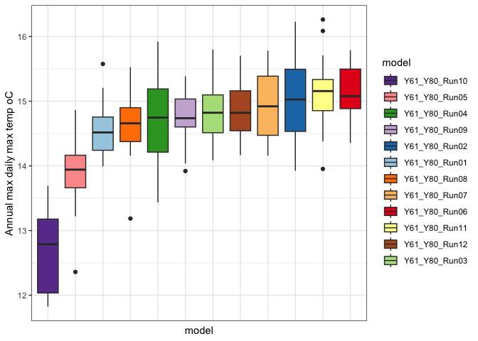
1.3.27 qqplot - annual means
ggplot(Y61_Y80_means_y, aes(sample=mean.annual, colour=factor(model))) +
  stat_qq() +
  stat_qq_line()+
  theme_bw()+
  scale_color_manual(values = my_colours) +
  facet_wrap(.~model, ncol=3)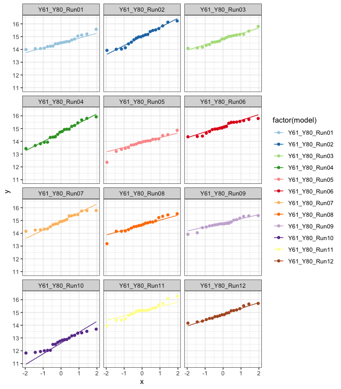
1.3.28 Time series - annual max
Y61_Y80_max_y <- Y61_Y80_means %>%
  group_by(Yf, model) %>%
dplyr::summarise(max=max(mean, na.rm=T))ggplot(Y61_Y80_max_y) +
geom_line(aes(x = as.numeric(Yf), y=max,
color=model)) +
theme_bw() + xlab("Year (2061 - 2080)") +
ylab("Annual max of mean daily max temp (tasmax) oC") +
scale_fill_brewer(palette = "Paired", name = "") +
scale_colour_brewer(palette = "Paired", name = "") +
theme(axis.text.x=element_blank(),
axis.ticks.x=element_blank())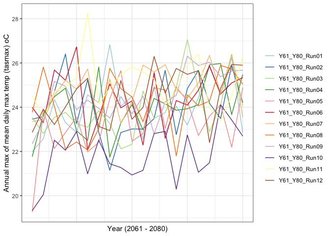
1.3.29 boxplot - annual max
Y61_Y80_max_y %>%
  mutate(model = fct_reorder(model, max, .fun='median')) %>%
    ggplot(aes(x=reorder(model, max), y=max, fill=model)) +
    geom_boxplot() + theme_bw() +
    ylab("Annual max of mean daily max temp (tasmax) oC") + xlab("model") +
   scale_fill_manual(values = my_colours) +
    theme(axis.text.x=element_blank(),
        axis.ticks.x=element_blank())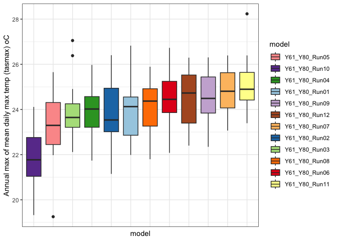
1.3.30 ANOVA
Daily means:
#-1 removes the intercept to compare coefficients of all Runs
av1 <- aov(mean ~ model - 1, Y61_Y80_means)
av1$coefficients[order(av1$coefficients)]
## modelY61_Y80_Run10 modelY61_Y80_Run05 modelY61_Y80_Run01 modelY61_Y80_Run08
## 12.70342 13.87016 14.55815 14.65973
## modelY61_Y80_Run04 modelY61_Y80_Run09 modelY61_Y80_Run03 modelY61_Y80_Run12
## 14.69527 14.76917 14.79545 14.87939
## modelY61_Y80_Run07 modelY61_Y80_Run02 modelY61_Y80_Run11 modelY61_Y80_Run06
## 14.94320 15.01577 15.11392 15.11814Annual means:
av2 <- aov(mean.annual ~ model - 1, Y61_Y80_means_y)
av2$coefficients[order(av2$coefficients)]
## modelY61_Y80_Run10 modelY61_Y80_Run05 modelY61_Y80_Run01 modelY61_Y80_Run08
## 12.70342 13.87016 14.55815 14.65973
## modelY61_Y80_Run04 modelY61_Y80_Run09 modelY61_Y80_Run03 modelY61_Y80_Run12
## 14.69527 14.76917 14.79545 14.87939
## modelY61_Y80_Run07 modelY61_Y80_Run02 modelY61_Y80_Run11 modelY61_Y80_Run06
## 14.94320 15.01577 15.11392 15.11814Max of means
av3 <- aov(max ~ model - 1, Y61_Y80_max_y)
av3$coefficients[order(av3$coefficients)]
## modelY61_Y80_Run10 modelY61_Y80_Run05 modelY61_Y80_Run03 modelY61_Y80_Run04
## 21.83290 23.32972 23.88512 23.98220
## modelY61_Y80_Run02 modelY61_Y80_Run01 modelY61_Y80_Run08 modelY61_Y80_Run06
## 23.98610 24.03094 24.13232 24.41824
## modelY61_Y80_Run12 modelY61_Y80_Run09 modelY61_Y80_Run07 modelY61_Y80_Run11
## 24.48810 24.53152 24.77651 25.09102Runs suggested by this slice are Run 05, Run 09, Run 03 and Run 11
Run 3 and 5 suggested above
1.4 3. Everything combined
The result per time slice suggest different runs, aside from run 5
1.4.1 Add in infill data
Update 13.05.23 - Adding in the infill data, and taking the anova result across the whole time period
Y <- rep(c(2001:2020), each=360)

dfs_Y00_Y20 <- lapply(names_Y00_Y20, function(i){
  df <- dfs_Y00_Y20[[i]]
  names(df) <- c("day", "mean", "sd")
  df$model <- i
  df$dn <- 1:nrow(df)
  df$Y <- Y
  df$Yf <- as.factor(df$Y)
  return(df)
})


Y <- rep(c(2041:2060), each=360)

dfs_Y41_Y60 <- lapply(names_Y41_Y60, function(i){
  df <- dfs_Y41_Y60[[i]]
  names(df) <- c("day", "mean", "sd")
  df$model <- i
  df$dn <- 1:nrow(df)
  df$Y <- Y
  df$Yf <- as.factor(df$Y)
  return(df)
})


#Create a single df in long form as above
Y00_Y20_means <- dfs_Y00_Y20 %>% reduce(rbind)
Y41_Y60_means <- dfs_Y41_Y60 %>% reduce(rbind)
Assessing what the combined times slices suggest via anova
1.4.1.1 Daily means:
#-1 removes the intercept to compare coefficients of all Runs
all.means <- rbind(historical_means, Y00_Y20_means, Y21_Y40_means, Y41_Y60_means, Y61_Y80_means)

x <- as.character(all.means$model)
all.means$model <- substr(x, nchar(x)-4, nchar(x))


av1 <- aov(mean ~ model - 1, all.means)
av1$coefficients[order(av1$coefficients)]
## modelRun10 modelRun05 modelRun09 modelRun04 modelRun03 modelRun07 modelRun08
## 11.12464 12.48165 12.79216 12.89910 12.91685 12.91894 12.95115
## modelRun02 modelRun01 modelRun12 modelRun06 modelRun11
## 12.95347 12.97947 13.38267 13.40644 13.611571.4.1.2 Annual means:
# As above, creating annual means
infill.L <- list(Y00_Y20_means, Y41_Y60_means)

infill.L_y <- lapply(infill.L, function(x){
  means_y <- x %>%
  group_by(Yf, model) %>%
  dplyr::summarise(mean.annual=mean(mean, na.rm=T), sd.annual=sd(mean, na.rm = T))})
## `summarise()` has grouped output by 'Yf'. You can override using the `.groups`
## argument.
## `summarise()` has grouped output by 'Yf'. You can override using the `.groups`
## argument.all.means_y <- rbind(historical_means_y,
infill.L_y[[1]],
Y21_Y40_means_y,
infill.L_y[[2]],
Y61_Y80_means_y)
x <- as.character(all.means_y$model)
all.means_y$model <- substr(x, nchar(x)-4, nchar(x))
av2 <- aov(mean.annual ~ model - 1, all.means_y)
av2$coefficients[order(av2$coefficients)]## modelRun10 modelRun05 modelRun09 modelRun04 modelRun03 modelRun07 modelRun08
## 11.12464 12.48165 12.79216 12.89910 12.91685 12.91894 12.95115
## modelRun02 modelRun01 modelRun12 modelRun06 modelRun11
## 12.95347 12.97947 13.38267 13.40644 13.61157Updated June 13th 2023 result
Considering all together, suggests: Runs 05, Run07, Run08 and Run06