Metrics¶

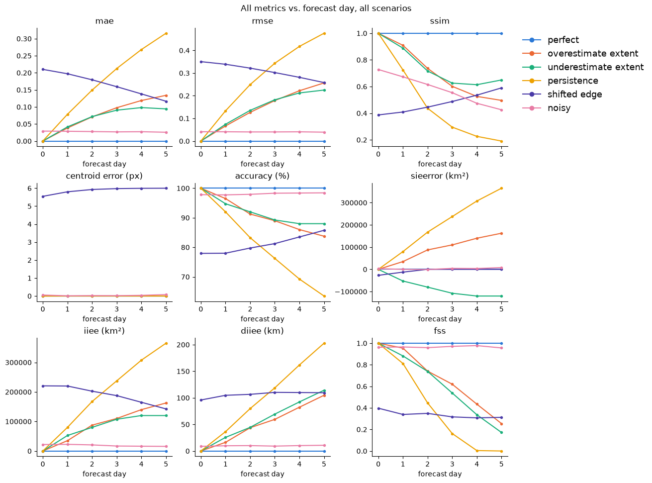
icenet_mp.metrics (API reference) implements several torchmetrics.Metric classes, each computed per forecast lead time. Using a combination of these metrics it is possible to understand why model results differ. Here we use six synthetic scenarios to show what each metric actually captures and what its strengths and weaknesses are.

Selecting which metrics run¶

Which metrics are computed during training, validation, and testing is controlled by the reporting.metrics Hydra config group.

uv run imp train --config-name <config> reporting.metrics="[accuracy,mae,rmse]"

or in a config file:

reporting:
  metrics:
    - accuracy
    - sieerror
    - fss_neighbourhood_size_5

The scenarios¶

All metrics below are computed against the same synthetic truth (a circular ice cap that shrinks over six forecast days, standing in for melt) and six prediction scenarios that implement a different type of error:

Metric summary¶

Continuous metrics¶

These are general-purpose metrics for comparing continuous fields, not specific to sea ice — most originate from image quality or regression evaluation and apply unchanged to any gridded continuous variable.

MAE / RMSE¶

MAEPerForecastDay and RMSEPerForecastDay compare concentration directly, pixel-by-pixel, independent of spatial pattern.

Limitations: Although these two produce similar rankings, RMSE weights large errors more than MAE, so it separates a few big misses (shifted edge) from many small ones (noisy) more sharply than MAE does. Neither metric distinguishes a coherent structural error from scattered noise with the same total magnitude — that distinction is what SSIM is for.

SSIM¶

SSIMPerForecastDay compares fields within a Gaussian-weighted window, combining local luminance, contrast, and structure (Wang et al., 2004), rather than comparing every pixel independently.

Limitations: SSIM is the one metric here that penalises noisy heavily (SSIM ≈ 0.58 averaged over the forecast) despite its low MAE/RMSE and high accuracy — independent per-pixel noise disrupts the local variance/covariance structure SSIM measures even though it averages out to a small mean error. It broadly agrees with most metrics that persistence and shifted edge are worst overall (both systematically wrong at every scale), but disagrees sharply on noisy, which most metrics rate as one of the best scenarios.

Centroid Error¶

CentroidErrorPerForecastDay measures the Euclidean distance, in pixels, between the value-weighted centroid ("center of mass") of the predicted and true fields — where the ice is, not how much of it there is.

Limitations: centroid error is blind to size bias by construction: growing or shrinking a circle around a fixed centre never moves its centre of mass, so overestimate extent, underestimate extent, and persistence all score ≈ 0 despite being some of the worst-performing scenarios by every area-based metric. shifted edge is the only scenario it penalises, converging toward the true 6-pixel displacement as the forecast progresses. Pair it with an area-based metric (SIE error, IIEE) to separate "wrong amount of ice" from "ice in the wrong place."

Spatial-mean trace¶

SpatialMeanGroundTruthPerForecastDay and SpatialMeanPredictionPerForecastDay each report the land-masked spatial mean of one field — the true concentration and the predicted concentration respectively — per forecast lead time. They are computed identically to every other PerForecastDay metric, and only differ in what they report: the field itself rather than an error between fields. Enabling both plots their traces together (they share the spatial_mean group, as fss_* does), so a systematic bias or a collapse toward a constant value shows up directly as the two traces pulling apart.

Limitations: like SIE error, the spatial mean is blind to spatial displacement — shifted edge has the same mean concentration as the truth throughout, so the two traces overlap despite the scenario being one of the worst by every other metric. It is not an error metric in its own right; pair it with MAE/RMSE or an area-based metric to see whether a matching mean also means a matching field.

Threshold-based (sea ice) metrics¶

These metrics have been developed specifically for quantifying errors in sea ice predictions. They work by first using a threshold (0.15 concentration) to get a binary ice/no-ice mask and then compare that, rather than the raw concentration.

Accuracy¶

IceNetAccuracyPerForecastDay reports the fraction of pixels that are correctly classified as either ice or no ice.

Limitations: accuracy only cares which side of the threshold a pixel lands on, not by how much. The noisy scenario scores 98 %+ despite non-zero MAE/RMSE, but shifted edge is penalised heavily (~81 % on average) since displaced ice pushes many pixels across the threshold in both directions.

SIE error¶

SeaIceExtentErrorPerForecastDay sums total ice area over the whole field and takes the signed difference from the truth. Positive means the model over-predicts extent.

Limitations: SIE error is blind to spatial displacement. shifted edge has the same total area as the truth every day, so its SIE error is near zero even though it is one of the worst scenarios by every other metric — area errors can cancel across the field even when the field is badly wrong locally. Combine it with a spatial metric such as IIEE, which does not let displacement errors cancel out.

IIEE¶

IntegratedIceEdgeErrorPerForecastDay measures the area of the symmetric difference between predicted and true ice extent (Goessling et al., 2016) — every disagreeing pixel counts, regardless of which side of the truth it's on.

Splitting the disagreement into an over-prediction area A (model says ice, truth says none) and an under-prediction area B (model says none, truth says ice) makes the relationship to SIE error explicit:

• SIE error = (A − B) × pixel area — a signed net difference, so A and B can cancel.
• IIEE = (A + B) × pixel area — an unsigned sum, so they never cancel.

IIEE is therefore always ≥ |SIEError|, with equality only when the disagreement is one-sided (A = 0 or B = 0).

Limitations: IIEE is a raw area, so its magnitude scales with domain size and total ice extent — a "good" IIEE for a large, heavily ice-covered domain is a different number than a "good" IIEE for a small or mostly ice-free one, even for equally skilled forecasts, so raw values aren't comparable across regions or seasons (DIIEE's edge-length normalisation exists to address this). IIEE also only reports how much area disagrees, not how that disagreement is distributed spatially: the same IIEE value can come from a small shift along a long, convoluted ice edge or a large shift along a short one, so it cannot be read as a literal displacement distance the way DIIEE can.

Interpreting alongside SIE error: the gap between the two is itself diagnostic. shifted edge has near-zero SIE error but the largest IIEE of any scenario, because the displacement creates an over-prediction region on one side of the truth and an under-prediction region on the other — A and B are both large but roughly equal, so they cancel in A − B while adding up unchanged in A + B. For pure area biases with no displacement (overestimate extent, underestimate extent, persistence), only one of A or B is non-zero, so IIEE tracks |SIEError| almost exactly. Report both together: if they're close, the model has a simple area bias; if IIEE is much larger, the total amount of ice is roughly right but it's in the wrong place — something SIE error alone would hide.

DIIEE¶

DistanceAveragedIceEdgeErrorPerForecastDay rescales IIEE into a length (km) by dividing by the combined predicted + true ice-edge length, giving a rough "average displacement" distance.

Limitations: DIIEE's denominator (combined edge length) is itself computed from the current prediction and truth, not a fixed constant like pixel_size — so it moves independently of the underlying error. A change in DIIEE from one lead time to the next can reflect a genuine change in forecast quality, a change in how much ice edge there is to normalise against, or both, and there is no way to tell which from DIIEE alone. DIIEE is also undefined (NaN) whenever both fields have no ice edge at all — fully ice-covered or fully ice-free — since the denominator is then zero. IIEE has no such gap: it is always well-defined and correctly reports 0 for a perfect match in that same case. This matters most near total melt or freeze-up, where DIIEE can go missing from a lead-time average exactly when IIEE keeps working.

Interpreting alongside IIEE: because its denominator is scenario- and time-dependent, DIIEE is not a fixed rescaling of IIEE — the two curves for the same scenario can have very different shapes. shifted edge illustrates this clearly: its IIEE declines steadily across the forecast (220,625 km² on day 0 down to 142,500 km² by day 5), which on its own looks like the forecast is improving, but its DIIEE stays within a narrow band around 110 km throughout. The displacement itself never changes — the ice cap is always offset sideways by the same fixed distance — what's actually happening is that the cap is simply melting and getting smaller, so there is less total area available to disagree over, which is enough on its own to shrink IIEE even though the underlying positional error hasn't improved at all DIIEE divides that same area by the combined edge length, which shrinks for the same reason, and this approximately cancels the "the whole cap is smaller now" effect out of the ratio — revealing that the actual displacement has stayed essentially constant rather than improved.

FSS¶

FractionalSkillScorePerForecastDay reduces each field to a binary ice-edge map, then compares the local fraction of edge cells within a neighbourhood_size × neighbourhood_size window (Roberts and Lean, 2008; Melsom et al., 2019). A small neighbourhood only forgives sub-pixel jitter; a large one forgives an edge displaced by many grid cells — computing FSS across a range of sizes and finding where it crosses 0.5 gives a rough "effective resolution" for edge position.

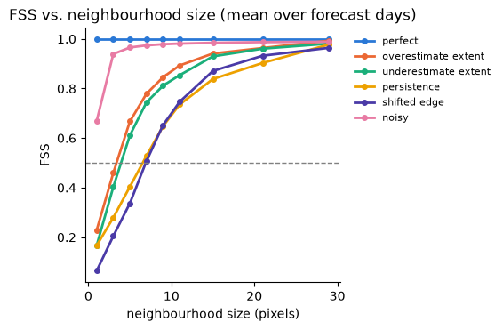
Limitations: FSS says nothing about how much concentration is wrong at a pixel, only whether the edge is in approximately the right place. noisy scores highest of any imperfect scenario (FSS ≈ 0.97 at a 5-pixel neighbourhood) since the edge survives small per-pixel noise almost perfectly, while persistence and shifted edge are the slowest to recover as the neighbourhood grows, since both are systematically — not just locally — wrong.

References¶

• Goessling, H. F., Tietsche, S., Day, J. J., Hawkins, E., and Jung, T. (2016). Predictability of the Arctic sea ice edge. Geophysical Research Letters, 43(4), 1642–1650. doi:10.1002/2015GL067232
• Melsom, A., Palerme, C., and Müller, M. (2019). Validation metrics for ice edge position forecasts. Ocean Science, 15, 615–630. doi:10.5194/os-15-615-2019
• Roberts, N. M., and Lean, H. W. (2008). Scale-Selective Verification of Rainfall Accumulations from High-Resolution Forecasts of Convective Events. Monthly Weather Review, 136(1), 78–97. doi:10.1175/2007MWR2123.1
• Wang, Z., Bovik, A. C., Sheikh, H. R., and Simoncelli, E. P. (2004). Image quality assessment: from error visibility to structural similarity. IEEE Transactions on Image Processing, 13(4), 600–612. doi:10.1109/TIP.2003.819861