10  The SPC pipeline

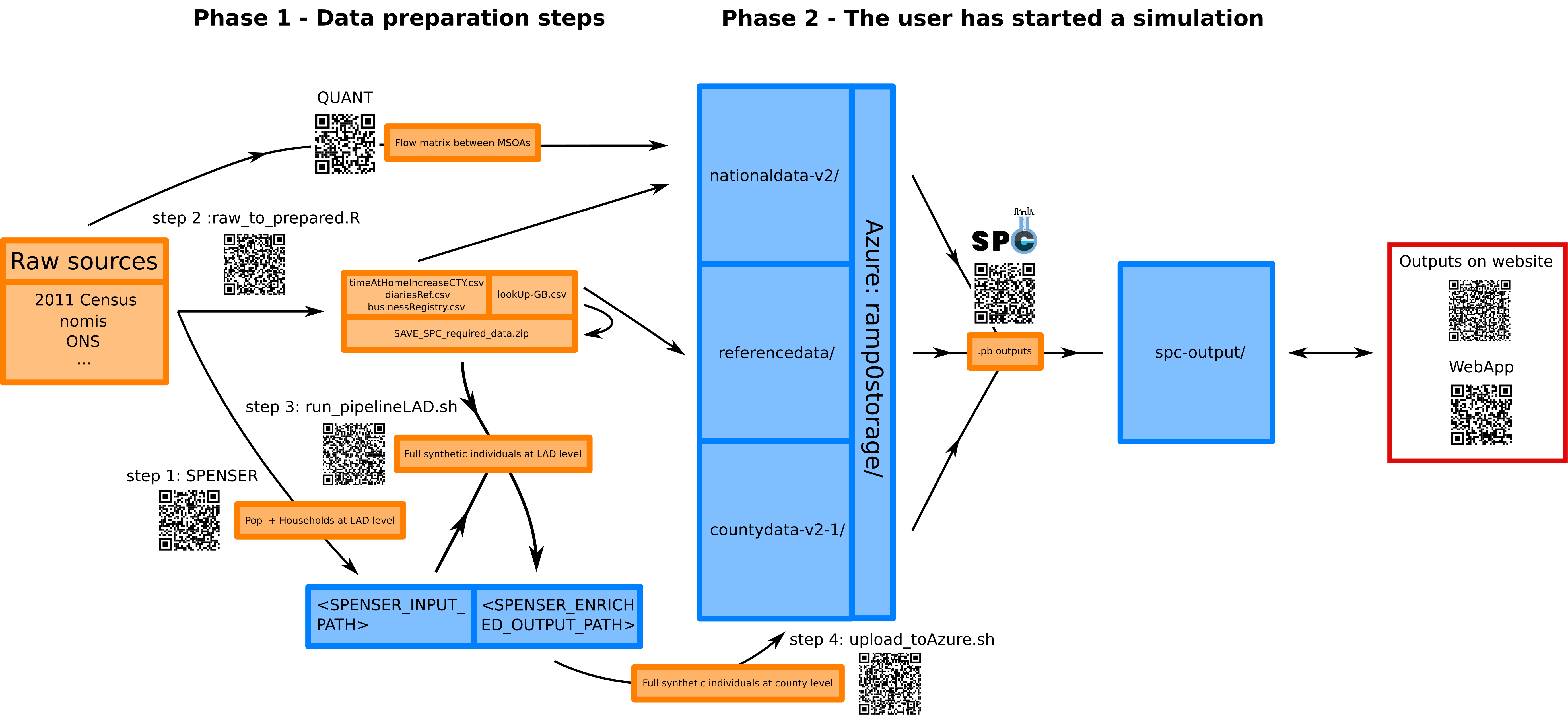
We provide in this document a step by step approach to running the entire SPC pipeline. This pipeline comprises the following steps.

• Phase 1 - Data preparation
  1. The SPENSER model creates a synthetic population with basic demographic information for all of GB.
  2. A script downloads and prepares data from various public sources that will be used throughout the model.
  3. The outputs of SPENSER are enriched using some of the outputs from step 2.
  4. The resulting outputs are uploaded as .csv files to a dedicated Azure repository.
• Phase 2 - The user has selected a study area and started a simulation
  1. All the data relevant to the study area are pulled from Azure.
  2. Individuals are assigned a single education destination (if under 16 y.o.) and several potential retail destinations, according to a local version of the QUANT model.
  3. Individuals are assigned a single workplace destination (if above 16 y.o), according to the method described here.
  4. The population, its activities and an optional lockdown modelling are gathered into a single .pb file that can be visualised with the SPC explorer.

We now explain how to run each step. The theoretical concepts supporting the modelling are presented here. The different data sources are detailed here.

10.1 Phase 1: Data preparation

10.1.1 SPENSER

The original SPENSER (Synthetic Population Estimation and Scenario Projection) model is made up of 5 different GitHub repositories, operating specific parts of the simulation of a synthetic population (gathering the data from ONS, creating individuals, creating households, assigning individuals to households and projecting the population to future years). We use this modified version with instructions for running the full pipeline on a single machine.

The SPENSER microsimulation is split into three steps:

1. Household synthesis: households are synthesised for a base year (2011) from census data at OA resolution. These households are then sequentially synthesised for subsequent years using household forecasts.
2. Population synthesis: people are sequentially synthesised using marginal census data on gender, age and ethnicity at MSOA resolution for 2011, with population projections used to derive the marginals beyond the reference census year.
3. Assignment: for a given year, a synthesised household (from step 1) is assigned to each member of the synthesised population (from step 2), while a “household representative person” from the synthesised population (from step 2) is assigned to each synthesised household (from step 1).

The result of SPENSER is two separate datasets and a merging key: one dataset for individuals, accurate at MSOA level and containing the sex, age and ethnicity fields; and one for households, accurate at OA level and containing the OA11CD, HOUSE_nssec8, House_type, HOUSE_typeCommunal, HOUSE_NRooms, HOUSE_centralHeat, HOUSE_tenure and HOUSE_NCars fields.

10.1.2 Downloading and preparation of public data from various sources

Instructions to run this step from the source code can be found under Step 1: Curate public data from diverse sources. More information on the various data sources can be found here. The result is a set of data files, some of which will be merged with the outputs from SPENSER during the next step, containing:

• NSSEC8 distributions among the population of England and Wales by age group and sex at MSOA level (NSSEC8_EW_F_16to24_CLEAN.csv, etc.) and among the total population of Scotland by age group, sex and ethnicity (NSSECS_CLEAN.csv)
• A combined extract from the three latest GB Health Surveys (HSComplete.csv)
• An extract from the UK Time Use Survey 2015 (indivTUS.csv)
• A file containing a set of coefficients to estimate the average BMI of individuals in England depending on their age, sex and ethnicity (BMIdMean.csv) and a file containing coefficients to obtain the equivalent average BMI in Scotland and Wales (BMIdiff.csv)
• Coefficients to estimate the hourly salary of an employee in England depending on their home region, sex, part-time/full-time status, age and SOC category (coefFFT.csv, etc. and ageRescaleFFT.csv, etc.).
• Coefficients to estimate the numbers of hours worked corresponding to the criteria mentioned above (meanHoursFFT.csv, etc. and distribHours.csv)
• Centroid coordinates of Output areas in GB (OACentroids.csv)

In addition, four files to be used by the second phase of the model are created:

• diariesRef.csv contains diaries of typical days extracted from the UK Time Use Survey
• businessRegistry.csv contains a list of all individual workplaces in GB
• timeAtHomeIncreaseCTY.csv contains a reduction in time spent away from home during the pandemic according to Google Mobility reports
• lookUp-GB.csv is a comprehensive lookup table between GB geographies, including name variants used by Google and OSM and local file names for storage within Azure

To understand the methods supporting the creation of these files, we refer the reader to the modelling methods section.

10.1.3 Enriching SPENSER

Instructions to run this step can be found under Step 2: Add to SPENSER. Line numbers quoted in the following refer to this script.

Once merged into one dataset according to the matching key (l. 13-49), the SPENSER data is enriched with the outputs of the previous step. An individual among those sharing the same 5-year age group (extra details for under 18) and sex is drawn (uniform distribution) from the participants of the Health Survey (l. 56-72). This adds the id_HS, HEALTH_diabetes, HEALTH_bloodpressure, HEALTH_cvd, HEALTH_NMedicines, HEALTH_selfAssessed and HEALTH_lifeSat fields. This join is not spatially differentiated and other potential matching criteria (such as ethnicity and nssec8) were not retained due to a lack of representativity for some groups inside the survey. The BMI field is then added l. 74-89, according to this method.

Each individual that is not a head of household is assigned an nssec8 category (l. 96-108). The probability distribution is given by nssec8 category distributions among the general population by sex and age groups according to ONS data (DC6114EW and DC6206SC datasets). An individual among those sharing the same 5-year age group, sex and nssec8 category is drawn (uniform distribution) from the participants of the UK Time Use Survey (l. 111-125). This adds the id_TUS_hh, id_TUS_p, pwkstat, soc2010, sic1d2007, sic2d2007, netPayWeekly and workedHoursWeekly fields. Note that the netPayWeekly and workedHoursWeekly fields had a low response rate among participants of the survey. For that reason, we have added a much more detailed modelling of income, that includes spatial differences at region level (l. 130-140).

Coordinates of the centroids of the OAs where the household’s home is located are finally added l. 152-156.

10.1.4 Azure upload

Following enrichment, a final step involves grouping LADs into counties and uploading to an Azure container for use as input for Phase 2 below.

10.2 Phase 2: Running SPC for a specific study area

This part is corresponding to the scripts written in Rust. Instructions can be found here.