A deeper dive into AutoEmulate#
Why AutoEmulate#
Simulations of real-world physical, chemical or biological processes can be complex and computationally expensive, and will often need high-performance computing resources and a lot of time to run. This becomes a problem when simulations need to be run thousands or tens of thousands of times to do uncertainty quantification or sensitivity analysis. It’s also a problem when a simulation needs to run fast enough to be useful in real-world or real-time applications, such as digital twins.
Emulator models are drop-in replacements for complex simulations, and can be orders of magnitude faster. Any model could be an emulator in principle, from a simple linear regression to Gaussian Processes to Neural Networks. Evaluating all these models requires time and machine learning expertise. AutoEmulate is designed to automate the process of finding a good emulator model for a simulation.
In the background, AutoEmulate does input processing, cross-validation, hyperparameter optimization and model selection. It’s different from typical AutoML packages, as the choice of models and hyperparameter search spaces is optimised for typical emulation problems. Over time, we expect the package to further adapt to the emulation needs of the community.
Workflow#
A typical workflow will involve
generating data from a simulation
running
AutoEmulatesummarising cross-validation results
refitting the emulator model on the full data
saving and loading the emulator.
import numpy as np
import pandas as pd
import matplotlib.pyplot as plt

from autoemulate.experimental_design import LatinHypercube
from autoemulate.simulations.epidemic import simulate_epidemic
from autoemulate.compare import AutoEmulate
1) Experimental Design (Sampling)#
Let’s first generate a set of inputs/outputs. We’ll use a simple simulator for the spread of infectious diseases based on the SIR model (see here for details). For simplicity, we assume a population size of 1000 individuals and start with 1 infected person. The simulator takes two inputs, the transmission rate per day and the recovery rate per day and outputs the peak infection rate.
We sample 200 sets of inputs X using a Latin Hypercube and run the simulator for those inputs to get a vector of outputs y.
seed = 42
np.random.seed(seed)

beta = (0.1, 0.5) # lower and upper bounds for the transmission rate
gamma = (0.01, 0.2) # lower and upper bounds for the recovery rate
lhd = LatinHypercube([beta, gamma])
X = lhd.sample(200)
y = np.array([simulate_epidemic(x) for x in X])

print(f"shapes: input X: {X.shape}, output y: {y.shape}\n")
print(f"X: {np.round(X[:3], 2)}\n")
print(f"y: {np.round(y[:3], 2)}\n")
shapes: input X: (200, 2), output y: (200,)

X: [[0.29 0.18]
 [0.13 0.04]
 [0.16 0.12]]

y: [0.09 0.31 0.03]
The general shape of the input data is a matrix X and a matrix (or vector) y where each row represents one run of the simulation and each column is a different input parameter. So in the example above, 0.29 and 0.18 are the two input parameters beta and gamma for the first run of the simulation, and 0.09 (peak transmission rate) is the output.
Note: The package currently only works with scalar inputs.
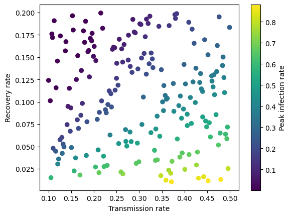
Let’s now plot the simulated data to see how the pattern looks like. As we might guess intuitively, the peak infection rate is higher when the transmission rate increases and the recovery rate decreases.
transmission_rate = X[:, 0]
recovery_rate = X[:, 1]

plt.scatter(transmission_rate, recovery_rate, c=y, cmap='viridis')
plt.xlabel('Transmission rate')
plt.ylabel('Recovery rate')
plt.colorbar(label="Peak infection rate")
plt.show
<function matplotlib.pyplot.show(close=None, block=None)>
2) Emulation#
A real world epidemic simulation will be computationally expensive and will take a long time to run. To evaluate the peak infection rate for thousands of different combinations of input parameters, it would be practical to to create a fast emulator model, which can then be used to predict the peak infection rate for new input parameters.
The simplest way to test different emulators is to run AutoEmulate with default parameters, providing only inputs X and outputs y. What happens in the background is that the inputs will be standardised (scale=True), after which various models are fitted and evaluated using 5-fold cross-validation.
em = AutoEmulate()
em.setup(X, y)
best_model = em.compare()
AutoEmulate is set up with the following settings:
| Values | |
|---|---|
| Simulation input shape (X) | (200, 2) |
| Simulation output shape (y) | (200,) |
| Proportion of data for testing (test_set_size) | 0.2 |
| Scale input data (scale) | True |
| Scaler (scaler) | StandardScaler |
| Scale output data (scale_output) | True |
| Scaler output (scaler_output) | StandardScaler |
| Do hyperparameter search (param_search) | False |
| Reduce input dimensionality (reduce_dim) | False |
| Reduce output dimensionality (reduce_dim_output) | False |
| Cross validator (cross_validator) | KFold |
| Parallel jobs (n_jobs) | 1 |
3) Summarising cross-validation results#
We can summarise the cross-validation results to see that several models have a high \(R^2\) and root mean squared error, suggesting a good fit. These metrics are the average metric on the test data across cv-folds.
em.summarise_cv()
| preprocessing | model | short | fold | rmse | r2 | |
|---|---|---|---|---|---|---|
| 0 | None | RadialBasisFunctions | rbf | 3 | 0.001507 | 0.999960 |
| 1 | None | GaussianProcess | gp | 3 | 0.002528 | 0.999889 |
| 2 | None | RadialBasisFunctions | rbf | 2 | 0.003658 | 0.999815 |
| 3 | None | GaussianProcess | gp | 2 | 0.003685 | 0.999813 |
| 4 | None | GaussianProcess | gp | 1 | 0.003307 | 0.999752 |
| 5 | None | RadialBasisFunctions | rbf | 0 | 0.003386 | 0.999744 |
| 6 | None | GaussianProcess | gp | 0 | 0.003802 | 0.999677 |
| 7 | None | GaussianProcess | gp | 4 | 0.006070 | 0.999413 |
| 8 | None | RadialBasisFunctions | rbf | 1 | 0.005182 | 0.999392 |
| 9 | None | RadialBasisFunctions | rbf | 4 | 0.011735 | 0.997808 |
| 10 | None | SupportVectorMachines | svm | 3 | 0.019997 | 0.993037 |
| 11 | None | SupportVectorMachines | svm | 0 | 0.017997 | 0.992765 |
| 12 | None | SupportVectorMachines | svm | 2 | 0.025602 | 0.990961 |
| 13 | None | GradientBoosting | gb | 4 | 0.023927 | 0.990885 |
| 14 | None | RandomForest | rf | 4 | 0.025527 | 0.989625 |
| 15 | None | SupportVectorMachines | svm | 1 | 0.023036 | 0.987986 |
| 16 | None | SecondOrderPolynomial | sop | 2 | 0.030193 | 0.987428 |
| 17 | None | GradientBoosting | gb | 2 | 0.030244 | 0.987386 |
| 18 | None | RandomForest | rf | 2 | 0.032616 | 0.985329 |
| 19 | None | RandomForest | rf | 0 | 0.027836 | 0.982693 |
| 20 | None | GradientBoosting | gb | 3 | 0.031541 | 0.982678 |
| 21 | None | SecondOrderPolynomial | sop | 0 | 0.028424 | 0.981954 |
| 22 | None | SupportVectorMachines | svm | 4 | 0.033742 | 0.981874 |
| 23 | None | GradientBoosting | gb | 1 | 0.028574 | 0.981514 |
| 24 | None | SecondOrderPolynomial | sop | 3 | 0.035508 | 0.978047 |
| 25 | None | LightGBM | lgbm | 3 | 0.037787 | 0.975138 |
| 26 | None | GradientBoosting | gb | 0 | 0.033802 | 0.974479 |
| 27 | None | RandomForest | rf | 3 | 0.039471 | 0.972873 |
| 28 | None | SecondOrderPolynomial | sop | 4 | 0.042687 | 0.970989 |
| 29 | None | LightGBM | lgbm | 0 | 0.037459 | 0.968657 |
| 30 | None | RandomForest | rf | 1 | 0.037461 | 0.968227 |
| 31 | None | LightGBM | lgbm | 1 | 0.038255 | 0.966865 |
| 32 | None | SecondOrderPolynomial | sop | 1 | 0.038917 | 0.965709 |
| 33 | None | LightGBM | lgbm | 2 | 0.059099 | 0.951832 |
| 34 | None | LightGBM | lgbm | 4 | 0.057692 | 0.947010 |
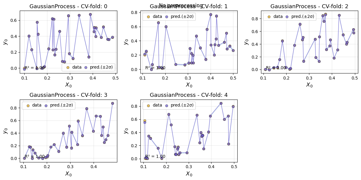
We can also look at each of the cv-folds for a specific model, like Gaussian Processes.
em.summarise_cv(model="GaussianProcess")
| preprocessing | model | short | fold | rmse | r2 | |
|---|---|---|---|---|---|---|
| 0 | None | GaussianProcess | gp | 3 | 0.002528 | 0.999889 |
| 1 | None | GaussianProcess | gp | 2 | 0.003685 | 0.999813 |
| 2 | None | GaussianProcess | gp | 1 | 0.003307 | 0.999752 |
| 3 | None | GaussianProcess | gp | 0 | 0.003802 | 0.999677 |
| 4 | None | GaussianProcess | gp | 4 | 0.006070 | 0.999413 |
Next, we can plot the cv results using different plot styles. If the simulation has multiple inputs and outputs, the default is to plot the first input (‘input_index=0’) and the first output (output_index=0), but this can be changed. The default style is Xy, which plots predictions and data points.
em.plot_cv()
Using best preprocessing method: None

No preprocessing was applied (using raw target values)
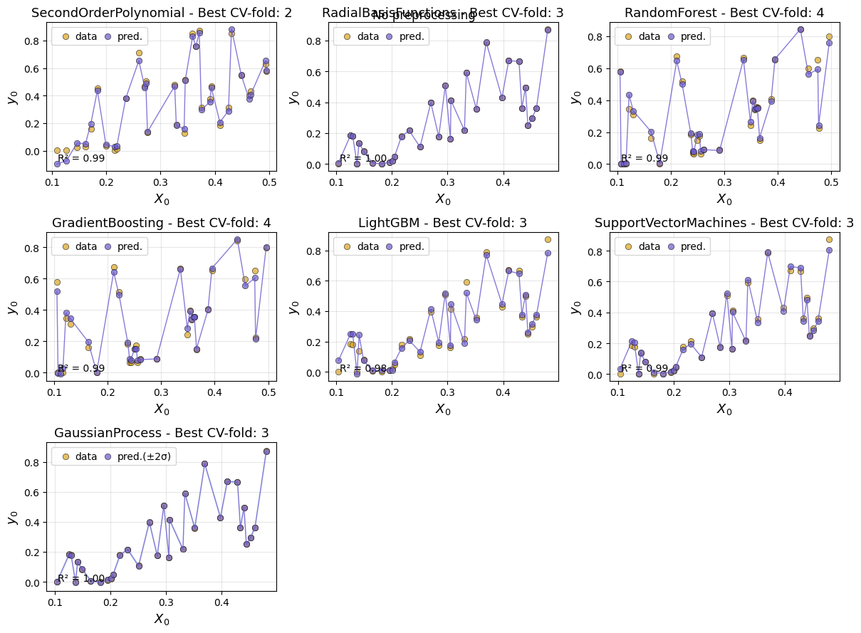
To inspect specific models more closely, we can plot the predictions for each cv fold for a given model.
em.plot_cv(model='GaussianProcess')
Using best preprocessing method: None

No preprocessing was applied (using raw target values)
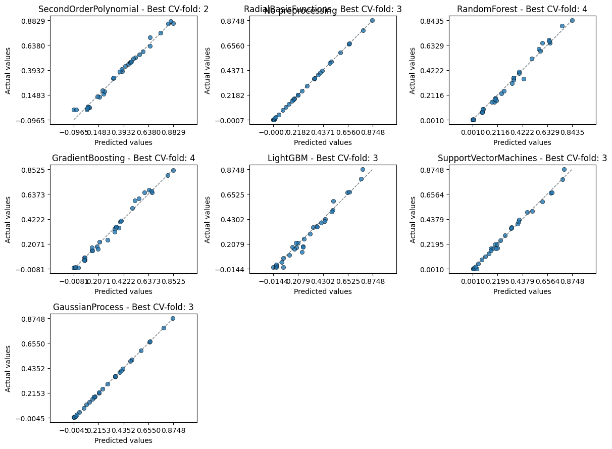
An alternative plot is actual_vs_predicted, which plots the true values against the predicted values.
em.plot_cv(style="actual_vs_predicted")
Using best preprocessing method: None

No preprocessing was applied (using raw target values)
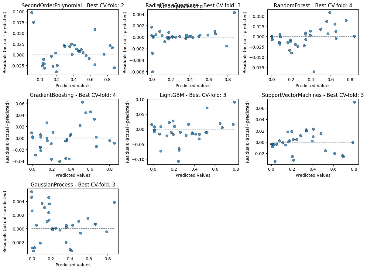
Always good to inspect the residuals too to spot any patterns.
em.plot_cv(style="residual_vs_predicted")
Using best preprocessing method: None

No preprocessing was applied (using raw target values)
5) Evaluate the emulator#
After looking at the cv results, we can chose an emulator model and see how it performs on the test-set, which AutoEmulate automatically sets aside.
gp = em.get_model("GaussianProcess")
em.evaluate(gp)
| model | short | preprocessing | rmse | r2 | |
|---|---|---|---|---|---|
| 0 | GaussianProcess | gp | None | 0.0027 | 0.9999 |
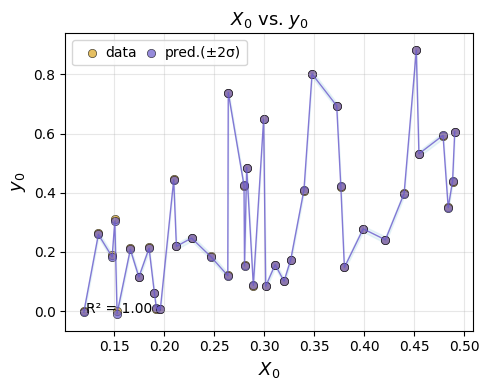
We can plot the test-set performance for chosen emulator.
em.plot_eval(gp)
4) Refitting the model on the full dataset#
AutoEmulate splits the dataset into a training and holdout set. All cross-validation, parameter optimisation and model selection is done on the training set. After we selected a best emulator model, we can refit it on the full dataset.
gp_final = em.refit(gp)
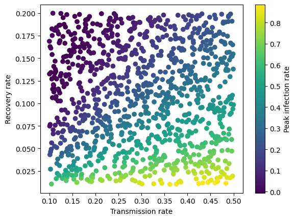
Let’s now try to predict the peak infection rate for a new set of transmission and recovery rates. Because our emulator is much faster then the original simulation, we can now evaluate the peak infection rate for a much larger set of input parameters.
seed = 42
np.random.seed(seed)

beta = (0.1, 0.5) # lower and upper bounds for the transmission rate
gamma = (0.01, 0.2) # lower and upper bounds for the recovery rate
lhd = LatinHypercube([beta, gamma])
X_new = lhd.sample(1000)
y_new = gp.predict(X_new)
And let’s do another plot:
transmission_rate = X_new[:, 0]
recovery_rate = X_new[:, 1]

plt.scatter(transmission_rate, recovery_rate, c=y_new, cmap='viridis')
plt.xlabel('Transmission rate')
plt.ylabel('Recovery rate')
plt.colorbar(label="Peak infection rate")
plt.show
<function matplotlib.pyplot.show(close=None, block=None)>
4) Saving / Loading#
We can save and load the model using em.save() and em.load(). The model is saved using joblib.dump. Next to the model, there is also a _meta.json file which specifies the required dependencies and should be present when loading the model to check that the correct package versions are installed.
# em.save(gp_final, "gp_final")
# gp_final_loaded = em.load("gp_final")
Hyperparameter search#
Although we tried to chose default model parameters that work well in a wide range of scenarios, hyperparameter search will often find an emulator model with a better fit. Internally, AutoEmulate compares the performance of different models and hyperparameters using cross-validation on the training data, which can be computationally expensive and time-consuming for larger datasets. To speed it up, we can parallelise the process with n_jobs.
For each model, we’ve pre-defined a search space for hyperparameters. When setting up AutoEmulate with param_search=True, we default to using random search with param_search_iters = 20 iterations. This means that 20 hyperparameter combinations from the search space are sampled and evaluated. We plan to add other hyperparameter search methods in the future.
Let’s do a hyperparameter search for the Support Vector Machines and Random Forest models.
em = AutoEmulate()
em.setup(X, y, param_search=True, param_search_type="random", param_search_iters=10, models=["SupportVectorMachines", "RandomForest"], n_jobs=-2) # n_jobs=-2 uses all cores but one
em.compare()
AutoEmulate is set up with the following settings:
| Values | |
|---|---|
| Simulation input shape (X) | (200, 2) |
| Simulation output shape (y) | (200,) |
| Proportion of data for testing (test_set_size) | 0.2 |
| Scale input data (scale) | True |
| Scaler (scaler) | StandardScaler |
| Scale output data (scale_output) | True |
| Scaler output (scaler_output) | StandardScaler |
| Do hyperparameter search (param_search) | True |
| Type of hyperparameter search (search_type) | random |
| Number of sampled parameter settings (param_search_iters) | 10 |
| Reduce input dimensionality (reduce_dim) | False |
| Reduce output dimensionality (reduce_dim_output) | False |
| Cross validator (cross_validator) | KFold |
| Parallel jobs (n_jobs) | -2 |
Pipeline(steps=[('scaler', StandardScaler()),
                ('model',
                 SupportVectorMachines(C=3.5738652727451714,
                                       coef0=0.7311573444549172, degree=5,
                                       epsilon=0.10339076097670674,
                                       gamma='auto', kernel='poly',
                                       tol=0.0002578733587284237))])
In a Jupyter environment, please rerun this cell to show the HTML representation or trust the notebook. On GitHub, the HTML representation is unable to render, please try loading this page with nbviewer.org.
Pipeline(steps=[('scaler', StandardScaler()),
                ('model',
                 SupportVectorMachines(C=3.5738652727451714,
                                       coef0=0.7311573444549172, degree=5,
                                       epsilon=0.10339076097670674,
                                       gamma='auto', kernel='poly',
tol=0.0002578733587284237))])StandardScaler()
SupportVectorMachines(C=3.5738652727451714, coef0=0.7311573444549172, degree=5,
                      epsilon=0.10339076097670674, gamma='auto', kernel='poly',
tol=0.0002578733587284237)em.summarise_cv()
| preprocessing | model | short | fold | rmse | r2 | |
|---|---|---|---|---|---|---|
| 0 | None | SupportVectorMachines | svm | 3 | 0.016816 | 0.995076 |
| 1 | None | SupportVectorMachines | svm | 2 | 0.019115 | 0.994961 |
| 2 | None | SupportVectorMachines | svm | 4 | 0.021872 | 0.992383 |
| 3 | None | SupportVectorMachines | svm | 0 | 0.019165 | 0.991796 |
| 4 | None | SupportVectorMachines | svm | 1 | 0.019038 | 0.991794 |
| 5 | None | RandomForest | rf | 4 | 0.028153 | 0.987381 |
| 6 | None | RandomForest | rf | 0 | 0.025734 | 0.985208 |
| 7 | None | RandomForest | rf | 2 | 0.035723 | 0.982401 |
| 8 | None | RandomForest | rf | 3 | 0.042547 | 0.968479 |
| 9 | None | RandomForest | rf | 1 | 0.038499 | 0.966441 |
Notes:
Some models, such as
GaussianProcesscan be slow when conducting hyperparameter search on larger datasets (say n > 1000).Use the
modelsargument to only run hyperparameter search on a subset of models to speed up the process.When possible, use
n_jobsto parallelise the hyperparameter search. With larger datasets, we recommend settingparam_search_itersto a lower number, such as 5, to see how long it takes to run and then increase it if necessary.all models can be specified with short names too, such as
rfforRandomForest,gpforGaussianProcess,svmforSupportVectorMachines, etc
Multioutput simulations#
All models run with multi-output data as well. Some models naively support multiple outputs. For models that don’t, AutoEmulate fits the model to each output separately under the hood. To see which models run separately for each output, we can check a model and see whether the pipeline includes a MultiOutputRegressor step. Note: all following metrics are averaged across outputs.
from autoemulate.simulations.projectile import simulate_projectile_multioutput
lhd = LatinHypercube([(-5., 1.), (0., 1000.)]) # (upper, lower) bounds for each parameter
X = lhd.sample(100)
y = np.array([simulate_projectile_multioutput(x) for x in X])
X.shape, y.shape
((100, 2), (100, 2))
em = AutoEmulate()
em.setup(X, y)
AutoEmulate is set up with the following settings:
| Values | |
|---|---|
| Simulation input shape (X) | (100, 2) |
| Simulation output shape (y) | (100, 2) |
| Proportion of data for testing (test_set_size) | 0.2 |
| Scale input data (scale) | True |
| Scaler (scaler) | StandardScaler |
| Scale output data (scale_output) | True |
| Scaler output (scaler_output) | StandardScaler |
| Do hyperparameter search (param_search) | False |
| Reduce input dimensionality (reduce_dim) | False |
| Reduce output dimensionality (reduce_dim_output) | False |
| Cross validator (cross_validator) | KFold |
| Parallel jobs (n_jobs) | 1 |
Custom standardisation, cross-validation and dimension reduction#
Standardisation#
AutoEmulate standardises inputs by default (scale=True) to have zero mean and unit variance. It uses scaler=StandardScaler() but other normalisers can be used, or the inputs can be left unscaled (scale=False). In addition, some models, like Gaussian Processes also standardise outputs, which makes them work better. Checking the parameters of a model with model.get_params() will show whether the model standardises outputs.
Dimension reduction#
When there are lots of input variables, it can be useful to reduce the dimensionality. To do this, we can add a dimension reduction step to each model using reduce_dim=True. By default, this uses PCA from scikit-learn, but other dimension reduction methods can be used.
Cross-validation#
The default cross-validation method is 5-fold cross-validation using sklearn.model_selection.KFold. The parameters can be changed or other cross-validation methods can be used, see sklearn.model_selection splitter classes for details.
Example#
Let’s say we wanted to change to a MinMaxScaler, to do PCA but retain components explaining more than 99% of the variance and do KFold cross validation but with 3 splits and no shuffling. To do this, we can just import the respective classes from sklearn and pass them to setup().
### Example
from sklearn.preprocessing import MinMaxScaler
from sklearn.decomposition import PCA
from sklearn.model_selection import KFold

mmscaler = MinMaxScaler()
pca = PCA(0.99)
kfold = KFold(n_splits=3, shuffle=False)

em = AutoEmulate()
em.setup(X, y, scale=True, scaler=mmscaler, cross_validator=kfold)
best_model = em.compare()
AutoEmulate is set up with the following settings:
| Values | |
|---|---|
| Simulation input shape (X) | (100, 2) |
| Simulation output shape (y) | (100, 2) |
| Proportion of data for testing (test_set_size) | 0.2 |
| Scale input data (scale) | True |
| Scaler (scaler) | MinMaxScaler |
| Scale output data (scale_output) | True |
| Scaler output (scaler_output) | StandardScaler |
| Do hyperparameter search (param_search) | False |
| Reduce input dimensionality (reduce_dim) | False |
| Reduce output dimensionality (reduce_dim_output) | False |
| Cross validator (cross_validator) | KFold |
| Parallel jobs (n_jobs) | 1 |
Note: Not all possible cross validators, scalers and decomposers have been tested and only a few make sense in the current version of AutoEmulate. If you encounter any issues, please open an issue on GitHub.
Downstream tasks#
Once you have a trained emulator, it can be used for many downstream tasks like sensitivity analysis or calibration. AutoEmulate comes with inbuilt support for some of the most common of these.
Sensitivity analysis#
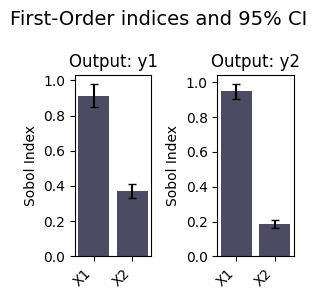
A common task for emulators is Global Sensitivity Analysis. We can perform this with the sensitivity_analysis method.
si = em.sensitivity_analysis(best_model)
si
| output | parameter | index | value | confidence | |
|---|---|---|---|---|---|
| 0 | y1 | X1 | S1 | 0.913411 | 0.132194 |
| 1 | y1 | X2 | S1 | 0.371139 | 0.084340 |
| 0 | y1 | X1 | ST | 0.630406 | 0.123627 |
| 1 | y1 | X2 | ST | 0.077955 | 0.056953 |
| 0 | y1 | [X1, X2] | S2 | 0.292805 | 0.217549 |
| 0 | y2 | X1 | S1 | 0.947820 | 0.086499 |
| 1 | y2 | X2 | S1 | 0.187317 | 0.047330 |
| 0 | y2 | X1 | ST | 0.812502 | 0.098226 |
| 1 | y2 | X2 | ST | 0.045686 | 0.030341 |
| 0 | y2 | [X1, X2] | S2 | 0.141774 | 0.144583 |
em.plot_sensitivity_analysis(si, index="S1", figsize=(3, 3))
