Data Requirements

Before getting started with DeepSensor, it’s important to understand the package’s data requirements. Further details on what DeepSensor supports and does not support are provided below.

DeepSensor does support:

• Arbitrary numbers of context sets (or data streams), each with arbitrary numbers of variables (i.e. data channels)

• Spatiotemporal data and static auxiliary data

• Gridded and off-the-grid data

• Moving sensors

• Missing data

DeepSensor does not support:

• Data with irregular temporal sampling (i.e. continuous time)

DeepSensor has the following data requirements:

• Data formats:

  • Pandas Series/DataFrame (i.e. tabular CSV data)

  • Xarray DataArray/Dataset (i.e. gridded NetCDF data)

• Regular temporal sampling (i.e. hourly, daily, monthly, etc.), which is the same for all variables

• Consistent spatiotemporal dimension names across variables (but arbitrary names are permitted, e.g. time, lat, lon, or date, y, x)

• Each variable has a unique ID, which is used to identify the variable in the model

• Missing data represented by NaNs (i.e., not arbitrary values such as -9999)

Data Sources

DeepSensor provides several functions in deepsensor.data.sources for fetching environmental data in the format expected by the package. These are not intended as definitive data sources for DeepSensor applications, but rather as a means of demoing and getting started with the package.

The following data sources are currently supported:

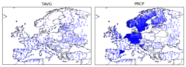
• GHCND: Global Historical Climatology Network Daily (GHCND) station data

• ERA5: ERA5 reanalysis data

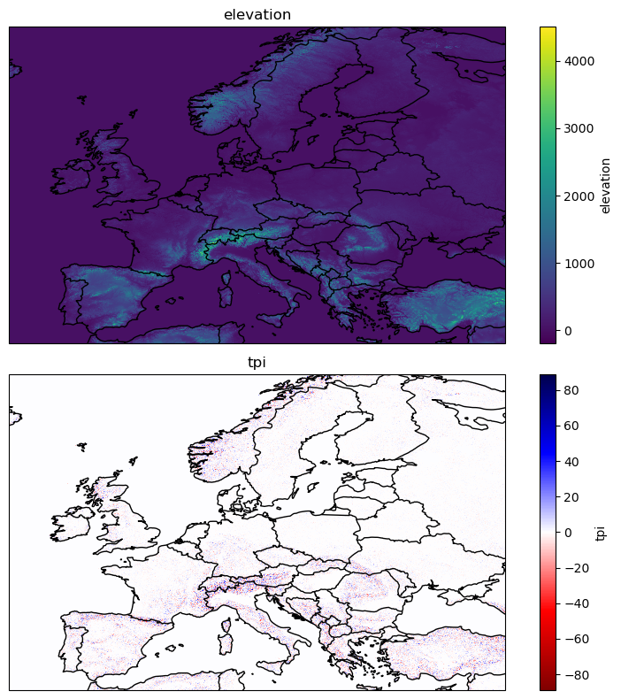
• EarthEnv: EarthEnv elevation and Topographic Position Index (TPI) data at various resolutions (1 km, 5 km, 10 km, 50 km, 100 km)

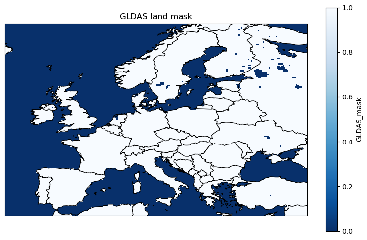
• GLDAS: Global Land Data Assimilation System (GLDAS) 0.25 degree resolution binary land mask

For more details on the data sources, see the API reference for the data.sources module.

Note

Some of the data downloader functions used here require additional dependencies. To run this yourself you will need to run:

pip install rioxarray

to install the rioxarray package and

pip install git+https://github.com/scott-hosking/get-station-data.git

to install the get_station_data package.

import logging
logging.captureWarnings(True)

import xarray as xr
import cartopy.crs as ccrs
import cartopy.feature as cfeature
import matplotlib.pyplot as plt

# Cache the data in root of docs/ folder, so that other notebook don't need to download it again
cache_dir = "../../.datacache"

from deepsensor.data.sources import get_ghcnd_station_data, get_era5_reanalysis_data, \
    get_earthenv_auxiliary_data, get_gldas_land_mask

data_range = ("2015-06-25", "2015-06-30")
extent = "europe"

Off-the-grid station data

Off-the-grid station data is data that is not on a regular grid, such as in-situ observations from weather stations. In DeepSensor, Pandas DataFrames are used to represent off-the-grid station data.

• The variable ID is the column name

• If the DataFrame has multiple columns, each column is treated as a separate variable

• The indexes must be (time, x1, x2), where time is a datetime, and x1 and x2 are the spatial dimensions

• There may be an arbitrary number of additional indexes after these first three indexes. This can be useful for tracking station IDs, for example.

station_var_IDs = ["TAVG", "PRCP"]
station_raw_df = get_ghcnd_station_data(station_var_IDs, extent, date_range=data_range, cache=True, cache_dir=cache_dir)
station_raw_df

				PRCP	TAVG
time	lat	lon	station
2015-06-25	35.017	-1.450	AGM00060531	0.0	23.0
	35.100	-1.850	AGE00147716	0.0	23.4
	35.117	36.750	SYM00040030	NaN	25.4
	35.167	2.317	AGM00060514	0.0	25.9
	35.200	-0.617	AGM00060520	0.0	24.9
...	...	...	...	...	...
2015-06-30	45.933	7.700	ITM00016052	NaN	5.7
	38.367	-0.500	SPM00008359	0.0	27.6
	55.383	36.700	RSM00027611	0.0	17.2
	59.080	17.860	SWE00138750	0.0	NaN
	63.760	12.430	SWE00140158	0.6	NaN

16922 rows × 2 columns

Show code cell source Hide code cell source

fig, axes = plt.subplots(1, len(station_var_IDs), subplot_kw={"projection": ccrs.PlateCarree()}, figsize=(4 * len(station_var_IDs), 4))
for ax, var_ID in zip(axes, station_var_IDs):
    df = station_raw_df[var_ID].dropna(how="any").reset_index()
    ax.scatter(df.lon, df.lat, transform=ccrs.PlateCarree(), color="b", marker="o", s=10, linewidth=0.1, facecolors='none')
    ax.coastlines(linewidths=0.5)
    ax.add_feature(cfeature.BORDERS, linewidths=0.5)
    ax.set_title(var_ID)
plt.tight_layout()

Spatiotemporal gridded data

Spatiotemporal gridded data is data that is on a regular spatiotemporal grid, such as reanalysis data or satellite data. In DeepSensor, Xarray DataArrays/Datasets are used to represent gridded data.

• The variable ID is the variable name in the DataArray/Dataset

• The dimensions must be (time, y, x), where time is a datetime, and y and x are the spatial dimensions

era5_var_IDs = ["2m_temperature", "10m_u_component_of_wind", "10m_v_component_of_wind"] 
era5_raw_ds = get_era5_reanalysis_data(era5_var_IDs, extent, date_range=data_range, cache=True, cache_dir=cache_dir)
era5_raw_ds 

<xarray.Dataset>
Dimensions:                  (time: 6, lat: 141, lon: 221)
Coordinates:
  * lat                      (lat) float32 70.0 69.75 69.5 ... 35.5 35.25 35.0
  * lon                      (lon) float32 -15.0 -14.75 -14.5 ... 39.75 40.0
  * time                     (time) datetime64[ns] 2015-06-25 ... 2015-06-30
Data variables:
    2m_temperature           (time, lat, lon) float32 274.7 274.8 ... 300.5
    10m_u_component_of_wind  (time, lat, lon) float32 5.999 5.951 ... 4.999
    10m_v_component_of_wind  (time, lat, lon) float32 2.87 2.746 ... -3.017

xarray.Dataset

• Dimensions:
  • time: 6
  • lat: 141
  • lon: 221
• Coordinates: (3)
  • lat
    (lat)
    float32
    70.0 69.75 69.5 ... 35.5 35.25 35.0

    long_name :

    latitude

    units :

    degrees_north

    array([70.  , 69.75, 69.5 , 69.25, 69.  , 68.75, 68.5 , 68.25, 68.  , 67.75,
           67.5 , 67.25, 67.  , 66.75, 66.5 , 66.25, 66.  , 65.75, 65.5 , 65.25,
           65.  , 64.75, 64.5 , 64.25, 64.  , 63.75, 63.5 , 63.25, 63.  , 62.75,
           62.5 , 62.25, 62.  , 61.75, 61.5 , 61.25, 61.  , 60.75, 60.5 , 60.25,
           60.  , 59.75, 59.5 , 59.25, 59.  , 58.75, 58.5 , 58.25, 58.  , 57.75,
           57.5 , 57.25, 57.  , 56.75, 56.5 , 56.25, 56.  , 55.75, 55.5 , 55.25,
           55.  , 54.75, 54.5 , 54.25, 54.  , 53.75, 53.5 , 53.25, 53.  , 52.75,
           52.5 , 52.25, 52.  , 51.75, 51.5 , 51.25, 51.  , 50.75, 50.5 , 50.25,
           50.  , 49.75, 49.5 , 49.25, 49.  , 48.75, 48.5 , 48.25, 48.  , 47.75,
           47.5 , 47.25, 47.  , 46.75, 46.5 , 46.25, 46.  , 45.75, 45.5 , 45.25,
           45.  , 44.75, 44.5 , 44.25, 44.  , 43.75, 43.5 , 43.25, 43.  , 42.75,
           42.5 , 42.25, 42.  , 41.75, 41.5 , 41.25, 41.  , 40.75, 40.5 , 40.25,
           40.  , 39.75, 39.5 , 39.25, 39.  , 38.75, 38.5 , 38.25, 38.  , 37.75,
           37.5 , 37.25, 37.  , 36.75, 36.5 , 36.25, 36.  , 35.75, 35.5 , 35.25,
           35.  ], dtype=float32)

  • lon
    (lon)
    float32
    -15.0 -14.75 -14.5 ... 39.75 40.0

    array([-15.  , -14.75, -14.5 , ...,  39.5 ,  39.75,  40.  ], dtype=float32)

  • time
    (time)
    datetime64[ns]
    2015-06-25 ... 2015-06-30

    array(['2015-06-25T00:00:00.000000000', '2015-06-26T00:00:00.000000000',
           '2015-06-27T00:00:00.000000000', '2015-06-28T00:00:00.000000000',
           '2015-06-29T00:00:00.000000000', '2015-06-30T00:00:00.000000000'],
          dtype='datetime64[ns]')

• Data variables: (3)
  • 2m_temperature
    (time, lat, lon)
    float32
    274.7 274.8 274.9 ... 300.1 300.5

    long_name :

    2 metre temperature

    short_name :

    t2m

    units :

    K

    array([[[274.66403, 274.77686, 274.87845, ..., 282.83322, 282.77402,
             282.68484],
            [274.87784, 274.9433 , 275.0187 , ..., 283.17734, 283.11746,
             283.0277 ],
            [275.16086, 275.22693, 275.29175, ..., 283.48465, 283.3743 ,
             283.28018],
            ...,
            [293.42294, 293.43103, 293.37308, ..., 301.89697, 302.78464,
             303.8855 ],
            [293.57944, 293.5258 , 293.446  , ..., 301.48306, 302.72665,
             304.24207],
            [293.60495, 293.56943, 293.49277, ..., 303.32947, 303.96527,
             304.5151 ]],
    
           [[275.19934, 275.27765, 275.3386 , ..., 281.7426 , 281.72858,
             281.72153],
            [275.76804, 275.77646, 275.79333, ..., 281.95264, 281.93762,
             281.93155],
            [276.31653, 276.3231 , 276.33014, ..., 282.16174, 282.1383 ,
             282.143  ],
    ...
            [293.3746 , 293.19507, 293.04773, ..., 300.4674 , 301.33984,
             302.3867 ],
            [293.3844 , 293.196  , 293.05753, ..., 300.13123, 301.37668,
             302.74155],
            [293.3275 , 293.20718, 293.09436, ..., 301.6532 , 302.2953 ,
             302.81848]],
    
           [[276.40662, 276.39536, 276.3816 , ..., 279.56448, 279.54074,
             279.53137],
            [276.46915, 276.426  , 276.4103 , ..., 279.7809 , 279.75717,
             279.74902],
            [276.6249 , 276.57736, 276.53168, ..., 279.95792, 279.9029 ,
             279.85788],
            ...,
            [293.995  , 293.90305, 293.83176, ..., 297.98416, 298.87292,
             299.9193 ],
            [294.0832 , 293.93182, 293.82925, ..., 297.87595, 299.09998,
             300.42343],
            [294.10632, 293.93558, 293.8136 , ..., 299.41083, 300.05502,
             300.53165]]], dtype=float32)

  • 10m_u_component_of_wind
    (time, lat, lon)
    float32
    5.999 5.951 5.912 ... 5.111 4.999

    long_name :

    10 metre U wind component

    short_name :

    u10

    units :

    m s**-1

    array([[[ 5.998557  ,  5.950816  ,  5.9116845 , ..., -1.4525173 ,
             -1.2940336 , -1.1206802 ],
            [ 6.125344  ,  6.129648  ,  6.1186914 , ..., -1.3816887 ,
             -1.22164   , -1.0467212 ],
            [ 6.1069517 ,  6.11243   ,  6.1190825 , ..., -1.5562164 ,
             -1.3977327 , -1.1774212 ],
            ...,
            [ 1.0119996 ,  1.0280436 ,  0.8108625 , ..., 11.532568  ,
             11.258646  , 10.319876  ],
            [ 1.156787  ,  0.92590976,  0.62772596, ..., 11.306778  ,
             11.148685  , 10.220089  ],
            [ 1.3892295 ,  0.9353014 ,  0.48998225, ..., 10.120695  ,
             10.185654  ,  9.932471  ]],
    
           [[ 6.625285  ,  6.741066  ,  6.8537793 , ...,  6.566244  ,
              6.541708  ,  6.496086  ],
            [ 6.153728  ,  6.275259  ,  6.3795385 , ...,  6.652505  ,
              6.6295023 ,  6.58273   ],
            [ 5.156557  ,  5.280772  ,  5.4061375 , ...,  6.631036  ,
              6.569695  ,  6.559727  ],
    ...
            [-0.33235008, -0.3066634 , -0.2599607 , ...,  6.500091  ,
              6.283821  ,  5.8437366 ],
            [-0.5096411 , -0.4796434 , -0.42306125, ...,  6.0380926 ,
              5.9188204 ,  5.402755  ],
            [-0.6228056 , -0.58310825, -0.5100003 , ...,  5.0621834 ,
              5.2292356 ,  5.184688  ]],
    
           [[-1.0508982 , -1.1892418 , -1.3131275 , ...,  8.129369  ,
              8.166259  ,  8.178971  ],
            [-1.6102542 , -1.6705769 , -1.7580696 , ...,  8.650336  ,
              8.688724  ,  8.700688  ],
            [-2.2568536 , -2.31593   , -2.3745077 , ...,  8.713402  ,
              8.84626   ,  8.899355  ],
            ...,
            [ 2.8763084 ,  2.7245045 ,  2.5455306 , ...,  6.698324  ,
              6.5019016 ,  5.99913   ],
            [ 2.571953  ,  2.404196  ,  2.2189903 , ...,  6.0771503 ,
              5.9879127 ,  5.4163423 ],
            [ 2.1447089 ,  2.0026264 ,  1.8453388 , ...,  5.001063  ,
              5.11099   ,  4.9985704 ]]], dtype=float32)

  • 10m_v_component_of_wind
    (time, lat, lon)
    float32
    2.87 2.746 2.627 ... -3.271 -3.017

    long_name :

    10 metre V wind component

    short_name :

    v10

    units :

    m s**-1

    array([[[ 2.8703592 ,  2.7455244 ,  2.6270146 , ...,  3.2172332 ,
              3.1672995 ,  3.1859415 ],
            [ 2.774819  ,  2.6709566 ,  2.5664282 , ...,  3.0704277 ,
              3.019495  ,  3.038137  ],
            [ 2.740531  ,  2.6353369 ,  2.5308087 , ...,  3.0404673 ,
              2.9469247 ,  2.929614  ],
            ...,
            [-2.6686413 , -2.2075853 , -1.8647058 , ..., -2.384351  ,
             -3.2804983 , -3.5185163 ],
            [-2.890348  , -2.511849  , -2.1340158 , ..., -4.663334  ,
             -4.403345  , -3.7089307 ],
            [-2.8643823 , -2.5917432 , -2.2778256 , ..., -3.980904  ,
             -3.069777  , -2.3250961 ]],
    
           [[ 4.2952785 ,  4.1775107 ,  4.0571113 , ...,  3.1478665 ,
              3.503143  ,  3.7024927 ],
            [ 4.3512015 ,  4.2492237 ,  4.124219  , ...,  3.6643333 ,
              4.0242157 ,  4.226197  ],
            [ 4.3459377 ,  4.2465925 ,  4.1459303 , ...,  4.1281667 ,
              4.349886  ,  4.5794992 ],
    ...
            [-4.3950157 , -4.7374463 , -5.1190586 , ..., -1.7439576 ,
             -2.3440766 , -2.4745612 ],
            [-4.5143833 , -4.8620987 , -5.2402487 , ..., -2.9999619 ,
             -2.963878  , -2.790749  ],
            [-4.596938  , -4.9493923 , -5.3069487 , ..., -2.6147046 ,
             -2.242933  , -2.0539494 ]],
    
           [[ 0.5779322 ,  0.5014291 ,  0.4173565 , ..., -3.2307386 ,
             -3.080435  , -2.8117275 ],
            [ 0.14324252,  0.01699861, -0.09005165, ..., -2.7492816 ,
             -2.5965455 , -2.3245945 ],
            [-0.23765151, -0.36632824, -0.49446455, ..., -2.2440364 ,
             -2.207001  , -2.0902185 ],
            ...,
            [ 0.6587607 ,  0.1808184 , -0.29550186, ..., -1.9880342 ,
             -2.5240974 , -2.6922424 ],
            [ 0.18379211, -0.1668253 , -0.61827534, ..., -3.5418875 ,
             -3.4759266 , -3.3010242 ],
            [-0.40849972, -0.66315   , -1.0467473 , ..., -3.733551  ,
             -3.2710173 , -3.0174484 ]]], dtype=float32)

• Indexes: (3)
  • lat
    PandasIndex

    PandasIndex(Index([ 70.0, 69.75,  69.5, 69.25,  69.0, 68.75,  68.5, 68.25,  68.0, 67.75,
           ...
           37.25,  37.0, 36.75,  36.5, 36.25,  36.0, 35.75,  35.5, 35.25,  35.0],
          dtype='float32', name='lat', length=141))

  • lon
    PandasIndex

    PandasIndex(Index([ -15.0, -14.75,  -14.5, -14.25,  -14.0, -13.75,  -13.5, -13.25,  -13.0,
           -12.75,
           ...
            37.75,   38.0,  38.25,   38.5,  38.75,   39.0,  39.25,   39.5,  39.75,
             40.0],
          dtype='float32', name='lon', length=221))

  • time
    PandasIndex

    PandasIndex(DatetimeIndex(['2015-06-25', '2015-06-26', '2015-06-27', '2015-06-28',
                   '2015-06-29', '2015-06-30'],
                  dtype='datetime64[ns]', name='time', freq='D'))

• Attributes: (0)

Show code cell source Hide code cell source

fig, axes = plt.subplots(1, len(era5_var_IDs), subplot_kw={"projection": ccrs.PlateCarree()}, figsize=(4 * len(era5_var_IDs), 3))
for ax, var_ID in zip(axes, era5_var_IDs):
    era5_raw_ds[var_ID].isel(time=0).plot(ax=ax, transform=ccrs.PlateCarree(), center=False, cmap="viridis")
    ax.coastlines()
    ax.add_feature(cfeature.BORDERS)
    ax.set_title(var_ID)
plt.tight_layout()

Static gridded data

We will often want to leverage static variables in our modelling pipelines. These static variables may provide information that aid predicting our target variables. For example, topography will affect surface temperature and soil type will affect soil moisture. DeepSensor classes support these ‘auxiliary’ variables with no time dimension. Here we will download 1 km resolution elevation and Topographic Position Index (TPI) data from EarthEnv, as well as a land mask from GLDAS.

auxiliary_var_IDs = ["elevation", "tpi"]
da = get_earthenv_auxiliary_data(auxiliary_var_IDs, extent, "1KM", cache=True, cache_dir=cache_dir)
da

<xarray.Dataset>
Dimensions:    (lon: 6600, lat: 4200)
Coordinates:
  * lon        (lon) float64 -15.0 -14.99 -14.98 -14.97 ... 39.98 39.99 40.0
  * lat        (lat) float64 70.0 69.99 69.98 69.97 ... 35.03 35.02 35.01 35.0
Data variables:
    elevation  (lat, lon) float32 0.0 0.0 0.0 0.0 ... 260.8 261.6 261.5 260.6
    tpi        (lat, lon) float32 0.0 0.0 0.0 0.0 ... 0.03906 0.07812 0.1641

xarray.Dataset

• Dimensions:
  • lon: 6600
  • lat: 4200
• Coordinates: (2)
  • lon
    (lon)
    float64
    -15.0 -14.99 -14.98 ... 39.99 40.0

    array([-14.995833, -14.9875  , -14.979167, ...,  39.979167,  39.9875  ,
            39.995833])

  • lat
    (lat)
    float64
    70.0 69.99 69.98 ... 35.01 35.0

    array([69.995833, 69.9875  , 69.979167, ..., 35.020833, 35.0125  , 35.004167])

• Data variables: (2)
  • elevation
    (lat, lon)
    float32
    0.0 0.0 0.0 ... 261.6 261.5 260.6

    array([[  0.    ,   0.    ,   0.    , ...,   0.    ,   0.    ,   0.    ],
           [  0.    ,   0.    ,   0.    , ...,   0.    ,   0.    ,   0.    ],
           [  0.    ,   0.    ,   0.    , ...,   0.    ,   0.    ,   0.    ],
           ...,
           [  0.    ,   0.    ,   0.    , ..., 261.9375, 262.5625, 261.4375],
           [  0.    ,   0.    ,   0.    , ..., 261.625 , 262.3125, 260.375 ],
           [  0.    ,   0.    ,   0.    , ..., 261.5625, 261.5   , 260.5625]],
          dtype=float32)

  • tpi
    (lat, lon)
    float32
    0.0 0.0 0.0 ... 0.07812 0.1641

    array([[ 0.       ,  0.       ,  0.       , ...,  0.       ,  0.       ,
             0.       ],
           [ 0.       ,  0.       ,  0.       , ...,  0.       ,  0.       ,
             0.       ],
           [ 0.       ,  0.       ,  0.       , ...,  0.       ,  0.       ,
             0.       ],
           ...,
           [ 0.       ,  0.       ,  0.       , ...,  0.3671875,  0.2421875,
             0.1171875],
           [ 0.       ,  0.       ,  0.       , ...,  0.1640625, -0.03125  ,
            -0.328125 ],
           [ 0.       ,  0.       ,  0.       , ...,  0.0390625,  0.078125 ,
             0.1640625]], dtype=float32)

• Indexes: (2)
  • lon
    PandasIndex

    PandasIndex(Index([-14.995833333333337, -14.987500000000011, -14.979166666666686,
           -14.970833333333331, -14.962500000000006,  -14.95416666666668,
           -14.945833333333326,            -14.9375, -14.929166666666674,
           -14.920833333333348,
           ...
             39.92083333333332,  39.929166666666646,             39.9375,
            39.945833333333326,   39.95416666666665,  39.962500000000006,
             39.97083333333333,   39.97916666666666,   39.98749999999998,
             39.99583333333334],
          dtype='float64', name='lon', length=6600))

  • lat
    PandasIndex

    PandasIndex(Index([ 69.99583333333334,  69.98750000000001,  69.97916666666667,
            69.97083333333333,            69.9625,  69.95416666666667,
            69.94583333333334,            69.9375,  69.92916666666667,
            69.92083333333333,
           ...
            35.07916666666667,  35.07083333333334,  35.06250000000001,
           35.054166666666674, 35.045833333333334,            35.0375,
            35.02916666666667, 35.020833333333336,            35.0125,
            35.00416666666667],
          dtype='float64', name='lat', length=4200))

• Attributes: (0)

Show code cell source Hide code cell source

fig, axes = plt.subplots(len(da.data_vars), 1, subplot_kw={"projection": ccrs.PlateCarree()}, figsize=(8, 4 * len(da.data_vars)))
for ax, var_ID in zip(axes, da.data_vars):
    if var_ID == "tpi":
        maxabs = max(abs(da[var_ID].min()), abs(da[var_ID].max()))
        da[var_ID].plot(ax=ax, transform=ccrs.PlateCarree(), cmap="seismic_r", vmin=-maxabs, vmax=maxabs)
    else:
        da[var_ID].plot(ax=ax, transform=ccrs.PlateCarree(), center=False, cmap="viridis")
    ax.coastlines()
    ax.add_feature(cfeature.BORDERS)
    ax.set_title(var_ID)
plt.tight_layout()

land_da = get_gldas_land_mask(extent, cache=True, cache_dir=cache_dir)
land_da

<xarray.DataArray 'GLDAS_mask' (lat: 140, lon: 220)>
array([[0., 0., 0., ..., 0., 0., 0.],
       [0., 0., 0., ..., 0., 0., 0.],
       [0., 0., 0., ..., 0., 0., 0.],
       ...,
       [0., 0., 0., ..., 1., 1., 1.],
       [0., 0., 0., ..., 1., 1., 1.],
       [0., 0., 0., ..., 1., 1., 1.]], dtype=float32)
Coordinates:
  * lon      (lon) float32 -14.88 -14.62 -14.38 -14.12 ... 39.38 39.62 39.88
  * lat      (lat) float32 69.88 69.62 69.38 69.12 ... 35.88 35.62 35.38 35.12

xarray.DataArray

'GLDAS_mask'

• lat: 140
• lon: 220

• 0.0 0.0 0.0 0.0 0.0 0.0 0.0 0.0 ... 1.0 1.0 1.0 1.0 1.0 1.0 1.0 1.0

  array([[0., 0., 0., ..., 0., 0., 0.],
         [0., 0., 0., ..., 0., 0., 0.],
         [0., 0., 0., ..., 0., 0., 0.],
         ...,
         [0., 0., 0., ..., 1., 1., 1.],
         [0., 0., 0., ..., 1., 1., 1.],
         [0., 0., 0., ..., 1., 1., 1.]], dtype=float32)

• Coordinates: (2)
  • lon
    (lon)
    float32
    -14.88 -14.62 ... 39.62 39.88

    units :

    degrees_east

    standard_name :

    longitude

    long_name :

    longitude

    vmin :

    -179.875

    vmax :

    179.875

    array([-14.875, -14.625, -14.375, ...,  39.375,  39.625,  39.875],
          dtype=float32)

  • lat
    (lat)
    float32
    69.88 69.62 69.38 ... 35.38 35.12

    units :

    degrees_north

    standard_name :

    latitude

    long_name :

    latitude

    vmin :

    -59.875

    vmax :

    89.875

    array([69.875, 69.625, 69.375, 69.125, 68.875, 68.625, 68.375, 68.125, 67.875,
           67.625, 67.375, 67.125, 66.875, 66.625, 66.375, 66.125, 65.875, 65.625,
           65.375, 65.125, 64.875, 64.625, 64.375, 64.125, 63.875, 63.625, 63.375,
           63.125, 62.875, 62.625, 62.375, 62.125, 61.875, 61.625, 61.375, 61.125,
           60.875, 60.625, 60.375, 60.125, 59.875, 59.625, 59.375, 59.125, 58.875,
           58.625, 58.375, 58.125, 57.875, 57.625, 57.375, 57.125, 56.875, 56.625,
           56.375, 56.125, 55.875, 55.625, 55.375, 55.125, 54.875, 54.625, 54.375,
           54.125, 53.875, 53.625, 53.375, 53.125, 52.875, 52.625, 52.375, 52.125,
           51.875, 51.625, 51.375, 51.125, 50.875, 50.625, 50.375, 50.125, 49.875,
           49.625, 49.375, 49.125, 48.875, 48.625, 48.375, 48.125, 47.875, 47.625,
           47.375, 47.125, 46.875, 46.625, 46.375, 46.125, 45.875, 45.625, 45.375,
           45.125, 44.875, 44.625, 44.375, 44.125, 43.875, 43.625, 43.375, 43.125,
           42.875, 42.625, 42.375, 42.125, 41.875, 41.625, 41.375, 41.125, 40.875,
           40.625, 40.375, 40.125, 39.875, 39.625, 39.375, 39.125, 38.875, 38.625,
           38.375, 38.125, 37.875, 37.625, 37.375, 37.125, 36.875, 36.625, 36.375,
           36.125, 35.875, 35.625, 35.375, 35.125], dtype=float32)

• Indexes: (2)
  • lon
    PandasIndex

    PandasIndex(Index([-14.875, -14.625, -14.375, -14.125, -13.875, -13.625, -13.375, -13.125,
           -12.875, -12.625,
           ...
            37.625,  37.875,  38.125,  38.375,  38.625,  38.875,  39.125,  39.375,
            39.625,  39.875],
          dtype='float32', name='lon', length=220))

  • lat
    PandasIndex

    PandasIndex(Index([69.875, 69.625, 69.375, 69.125, 68.875, 68.625, 68.375, 68.125, 67.875,
           67.625,
           ...
           37.375, 37.125, 36.875, 36.625, 36.375, 36.125, 35.875, 35.625, 35.375,
           35.125],
          dtype='float32', name='lat', length=140))

• Attributes: (0)

Show code cell source Hide code cell source

fig, ax = plt.subplots(1, 1, subplot_kw={"projection": ccrs.PlateCarree()}, figsize=(8, 5))
land_da.plot(ax=ax, transform=ccrs.PlateCarree(), center=False, cmap="Blues_r")
ax.coastlines()
ax.add_feature(cfeature.BORDERS)
ax.set_title("GLDAS land mask")
plt.tight_layout()