Prediction

DeepSensor provides a convenient high-level interface to predict directly to xarray or pandas objects in the original units and coordinate system of your data. This is achieved using the model.predict method. We’ll use our trained model from the Training page to demonstrate DeepSensor’s prediction functionality.

The two key arguments of model.predict are 1) a Task (or list of Tasks) containing context data, and 2) a set of target prediction locations, X_t. This page will demonstrate how we can predict on-grid or off-grid based on the form of X_t. We will also see how we can use optional extra arguments in model.predict for more advanced usage.

Show code cell content

Hide code cell content

import logging
logging.captureWarnings(True)

import deepsensor.torch
from deepsensor.model import ConvNP
from deepsensor.train import Trainer, set_gpu_default_device
from deepsensor.data import DataProcessor, TaskLoader, construct_circ_time_ds
from deepsensor.data.sources import get_era5_reanalysis_data, get_earthenv_auxiliary_data, get_gldas_land_mask

import xarray as xr
import cartopy.crs as ccrs
import matplotlib.pyplot as plt
import pandas as pd
import numpy as np
from tqdm import tqdm_notebook

Show code cell content

Hide code cell content

# Training/data config
data_range = ("2010-01-01", "2019-12-31")
train_range = ("2010-01-01", "2018-12-31")
val_range = ("2019-01-01", "2019-12-31")
date_subsample_factor = 2
extent = "north_america"
era5_var_IDs = ["2m_temperature"]
lowres_auxiliary_var_IDs = ["elevation"]
cache_dir = "../../.datacache"
deepsensor_folder = "../deepsensor_config/"
verbose_download = True

Show code cell content

Hide code cell content

era5_raw_ds = get_era5_reanalysis_data(era5_var_IDs, extent, date_range=data_range, cache=True, cache_dir=cache_dir, verbose=verbose_download, num_processes=8)
lowres_aux_raw_ds = get_earthenv_auxiliary_data(lowres_auxiliary_var_IDs, extent, "100KM", cache=True, cache_dir=cache_dir, verbose=verbose_download)
land_mask_raw_ds = get_gldas_land_mask(extent, cache=True, cache_dir=cache_dir, verbose=verbose_download)

data_processor = DataProcessor(x1_name="lat", x2_name="lon")
era5_ds = data_processor(era5_raw_ds)
lowres_aux_ds, land_mask_ds = data_processor([lowres_aux_raw_ds, land_mask_raw_ds], method="min_max")

dates = pd.date_range(era5_ds.time.values.min(), era5_ds.time.values.max(), freq="D")
doy_ds = construct_circ_time_ds(dates, freq="D")
lowres_aux_ds["cos_D"] = doy_ds["cos_D"]
lowres_aux_ds["sin_D"] = doy_ds["sin_D"]

Downloading ERA5 data from Google Cloud Storage... 

100%|██████████████████████████████████████████████████████████████████| 120/120 [00:04<00:00, 25.63it/s]

1.41 GB loaded in 7.09 s

task_loader = TaskLoader(
    context=[era5_ds, land_mask_ds, lowres_aux_ds],
    target=era5_ds,
)
task_loader.load_dask()
print(task_loader)

TaskLoader(3 context sets, 1 target sets)
Context variable IDs: (('2m_temperature',), ('GLDAS_mask',), ('elevation', 'cos_D', 'sin_D'))
Target variable IDs: (('2m_temperature',),)

set_gpu_default_device()

# Set up model
model = ConvNP(data_processor, task_loader, deepsensor_folder)

Predict on-grid to xarray

If X_t is an xarray object, model.predict will return xarray predictions on the same grid as that object (with the resolution optionally scaled by resolution_factor).

date = "2019-06-25"
test_task = task_loader(date, [100, "all", "all"], seed_override=42)
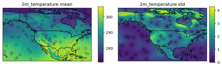
pred = model.predict(test_task, X_t=era5_raw_ds, resolution_factor=2)

The result is a single dictionary-like Prediction object whose keys are the variable IDs of the target variables, each mapping to xarray.Dataset objects containing the prediction parameters (in this case the mean and std of the ConvNP’s Gaussian likelihood).

pred["2m_temperature"]

<xarray.Dataset>
Dimensions:  (time: 1, lat: 482, lon: 802)
Coordinates:
  * lat      (lat) float64 75.0 74.88 74.75 74.63 ... 15.37 15.25 15.12 15.0
  * lon      (lon) float64 -160.0 -159.9 -159.8 -159.6 ... -60.25 -60.12 -60.0
  * time     (time) datetime64[ns] 2019-06-25
Data variables:
    mean     (time, lat, lon) float32 275.0 275.2 275.1 ... 300.9 300.9 301.1
    std      (time, lat, lon) float32 1.811 1.665 1.554 ... 0.6224 0.629 0.6557

xarray.Dataset

• Dimensions:
  • time: 1
  • lat: 482
  • lon: 802
• Coordinates: (3)
  • lat
    (lat)
    float64
    75.0 74.88 74.75 ... 15.12 15.0

    long_name :

    latitude

    units :

    degrees_north

    array([75.     , 74.87526, 74.75052, ..., 15.24948, 15.12474, 15.     ])

  • lon
    (lon)
    float64
    -160.0 -159.9 ... -60.12 -60.0

    array([-160.      , -159.875156, -159.750312, ...,  -60.249688,  -60.124844,
            -60.      ])

  • time
    (time)
    datetime64[ns]
    2019-06-25

    array(['2019-06-25T00:00:00.000000000'], dtype='datetime64[ns]')

• Data variables: (2)
  • mean
    (time, lat, lon)
    float32
    275.0 275.2 275.1 ... 300.9 301.1

    array([[[275.00452, 275.22607, 275.11514, ..., 274.93878, 275.45047,
             276.25586],
            [274.97293, 275.1751 , 275.07507, ..., 275.02182, 275.5157 ,
             276.31436],
            [274.72708, 274.90143, 274.82806, ..., 275.05002, 275.48322,
             276.2145 ],
            ...,
            [300.7698 , 300.40784, 300.24695, ..., 300.4926 , 300.48068,
             300.69186],
            [300.8241 , 300.47003, 300.31256, ..., 300.61224, 300.5973 ,
             300.80008],
            [300.80624, 300.47333, 300.33188, ..., 300.8911 , 300.88892,
             301.08026]]], dtype=float32)

  • std
    (time, lat, lon)
    float32
    1.811 1.665 1.554 ... 0.629 0.6557

    array([[[1.8110253 , 1.66512   , 1.5535779 , ..., 1.2972987 ,
             1.4221095 , 1.5792123 ],
            [1.6006852 , 1.4761493 , 1.3834654 , ..., 1.1284314 ,
             1.2286643 , 1.3568451 ],
            [1.4599366 , 1.3524946 , 1.2756103 , ..., 1.0287951 ,
             1.110107  , 1.2157164 ],
            ...,
            [0.7947206 , 0.7175477 , 0.674785  , ..., 0.58165216,
             0.5893423 , 0.61390746],
            [0.87569636, 0.78372097, 0.7296483 , ..., 0.59439784,
             0.60126275, 0.6265266 ],
            [1.0000812 , 0.8869281 , 0.8163588 , ..., 0.6224214 ,
             0.62899923, 0.6557162 ]]], dtype=float32)

• Indexes: (3)
  • lat
    PandasIndex

    PandasIndex(Index([              75.0,  74.87525987525987,  74.75051975051976,
            74.62577962577963,   74.5010395010395,  74.37629937629937,
            74.25155925155926,  74.12681912681913,    74.002079002079,
            73.87733887733887,
           ...
            16.12266112266112, 15.997920997920993, 15.873180873180871,
           15.748440748440743, 15.623700623700621, 15.498960498960493,
           15.374220374220371, 15.249480249480243, 15.124740124740121,
                         15.0],
          dtype='float64', name='lat', length=482))

  • lon
    PandasIndex

    PandasIndex(Index([             -160.0, -159.87515605493132, -159.75031210986268,
             -159.625468164794, -159.50062421972535, -159.37578027465668,
             -159.250936329588, -159.12609238451935, -159.00124843945068,
           -158.87640449438203,
           ...
           -61.123595505617985,  -60.99875156054931,  -60.87390761548065,
           -60.749063670411985,  -60.62421972534332,  -60.49937578027466,
              -60.374531835206, -60.249687890137324,  -60.12484394506866,
                         -60.0],
          dtype='float64', name='lon', length=802))

  • time
    PandasIndex

    PandasIndex(DatetimeIndex(['2019-06-25'], dtype='datetime64[ns]', name='time', freq=None))

• Attributes: (0)

fig = deepsensor.plot.prediction(pred, date, data_processor, task_loader, test_task, crs=ccrs.PlateCarree())

Predict off-grid to pandas

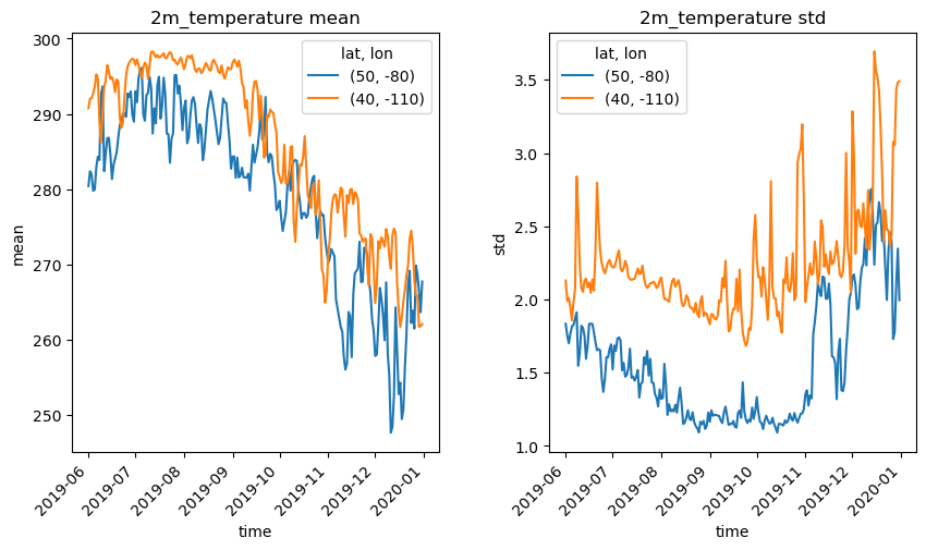
Predicting at off-grid locations with model.predict is very similar to the on-grid case above. If X_t is 1) a shape \((2, N)\) numpy array, or 2) a pandas object containing spatial indexes, the values of the Prediction returned by model.predict will be pandas.DataFrames whose columns are the prediction parameters.

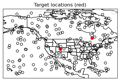
Let’s see an example where we pass a list of Tasks to model.predict, with context sets spanning the second half of 2019. Check out the indexes of the resulting pandas.DataFrame!

# Predict at two off-grid locations over six months of 2019 with 200 random context points (fixed across time)
test_tasks = task_loader(pd.date_range("2019-06-01", "2019-12-31"), [200, "all", "all"], seed_override=42)
X_t = np.array([[50, -80],
                [40, -110]]).T
pred = model.predict(test_tasks, X_t=X_t)

# plot the target locations and the context locations on a map
fig, ax = plt.subplots(figsize=(5, 5), subplot_kw={"projection": ccrs.PlateCarree()})
deepsensor.plot.offgrid_context(ax, test_tasks[0], data_processor, task_loader)
ax.scatter(X_t[1], X_t[0], c="r", s=50)
ax.coastlines()
ax.set_title("Target locations (red)")
ax.add_feature(ccrs.cartopy.feature.STATES)

No artists with labels found to put in legend.  Note that artists whose label start with an underscore are ignored when legend() is called with no argument.

<cartopy.mpl.feature_artist.FeatureArtist at 0x7fd4927df650>

pred["2m_temperature"]

			mean	std
time	lat	lon
2019-06-01	50	-80	280.406281	1.834735
	40	-110	290.741547	2.129284
2019-06-02	50	-80	282.370087	1.753442
	40	-110	292.015839	1.990584
2019-06-03	50	-80	281.934479	1.701114
...	...	...	...	...
2019-12-29	40	-110	261.715698	3.435812
2019-12-30	50	-80	263.644775	2.347633
	40	-110	261.7883	3.48374
2019-12-31	50	-80	267.722748	1.995918
	40	-110	262.06546	3.490994

428 rows × 2 columns

fig = deepsensor.plot.prediction(pred)

Advanced: Autoregressive sampling

The model.predict method supports autoregressive (AR) sampling, which is useful for generating spatially correlated samples. AR sampling works by passing model samples at target points back into the model as context points. In model.predict, this is achieved by passing n_samples > 0 with ar_sample.

AR sampling can be computationally expensive because it requires a forward pass of the model for each target point. DeepSensor provides functionality to draw cheaper AR samples only over a subset of target points, and then interpolate those samples with a single forward pass of the model. This is achieved using by passing an integer ar_subsample_factor > 1. X_t will be subsampled by a factor of ar_subsample_factor in both spatial dimensions to obtain the AR sample locations. Note, subsampling will result in a loss of spatial granularity in the AR samples.

For more information, check out the Autoregressive Conditional Neural Processes paper (ICLR, 2023).

date = "2019-06-25"
test_task = task_loader(date, [100, "all", "all"], seed_override=42)
X_t = era5_raw_ds
pred = model.predict(test_task, X_t=X_t, n_samples=3, ar_sample=True, ar_subsample_factor=10)

pred["2m_temperature"]

<xarray.Dataset>
Dimensions:   (time: 1, lat: 241, lon: 401)
Coordinates:
  * lat       (lat) float32 75.0 74.75 74.5 74.25 74.0 ... 15.75 15.5 15.25 15.0
  * lon       (lon) float32 -160.0 -159.8 -159.5 -159.2 ... -60.5 -60.25 -60.0
  * time      (time) datetime64[ns] 2019-06-25
Data variables:
    mean      (time, lat, lon) float32 275.0 275.1 274.4 ... 301.0 300.9 301.1
    std       (time, lat, lon) float32 1.811 1.553 1.384 ... 0.6224 0.6557
    sample_0  (time, lat, lon) float32 275.8 274.9 273.8 ... 302.4 302.7 303.6
    sample_1  (time, lat, lon) float32 274.5 273.8 272.9 ... 302.5 302.8 303.7
    sample_2  (time, lat, lon) float32 276.8 275.8 274.5 ... 302.5 302.7 303.7

xarray.Dataset

• Dimensions:
  • time: 1
  • lat: 241
  • lon: 401
• Coordinates: (3)
  • lat
    (lat)
    float32
    75.0 74.75 74.5 ... 15.5 15.25 15.0

    long_name :

    latitude

    units :

    degrees_north

    array([75.  , 74.75, 74.5 , ..., 15.5 , 15.25, 15.  ], dtype=float32)

  • lon
    (lon)
    float32
    -160.0 -159.8 ... -60.25 -60.0

    array([-160.  , -159.75, -159.5 , ...,  -60.5 ,  -60.25,  -60.  ],
          dtype=float32)

  • time
    (time)
    datetime64[ns]
    2019-06-25

    array(['2019-06-25T00:00:00.000000000'], dtype='datetime64[ns]')

• Data variables: (5)
  • mean
    (time, lat, lon)
    float32
    275.0 275.1 274.4 ... 300.9 301.1

    array([[[275.00452, 275.1145 , 274.3951 , ..., 274.52783, 274.93784,
             276.25586],
            [274.72586, 274.82635, 274.31317, ..., 274.7952 , 275.04935,
             276.21387],
            [274.22696, 274.27237, 273.94662, ..., 274.99216, 275.05637,
             275.8078 ],
            ...,
            [300.53406, 300.0763 , 299.9431 , ..., 300.62006, 300.55438,
             300.79172],
            [300.76944, 300.24637, 300.166  , ..., 300.70886, 300.49265,
             300.6917 ],
            [300.80624, 300.3317 , 300.3061 , ..., 301.0215 , 300.89127,
             301.08026]]], dtype=float32)

  • std
    (time, lat, lon)
    float32
    1.811 1.553 1.384 ... 0.6224 0.6557

    array([[[1.8110253 , 1.553329  , 1.384296  , ..., 1.1187122 ,
             1.2970232 , 1.5792123 ],
            [1.4594713 , 1.275099  , 1.1630592 , ..., 0.91676354,
             1.0283178 , 1.2152662 ],
            [1.3194875 , 1.1786841 , 1.1037246 , ..., 0.8871782 ,
             0.9590363 , 1.0891011 ],
            ...,
            [0.71183395, 0.6217848 , 0.6075412 , ..., 0.57358634,
             0.5719306 , 0.6060664 ],
            [0.7944542 , 0.6745316 , 0.6408484 , ..., 0.58629495,
             0.5816154 , 0.6138778 ],
            [1.0000812 , 0.81622076, 0.74212545, ..., 0.6326938 ,
             0.6224225 , 0.6557162 ]]], dtype=float32)

  • sample_0
    (time, lat, lon)
    float32
    275.8 274.9 273.8 ... 302.7 303.6

    array([[[275.83643, 274.94324, 273.786  , ..., 274.38947, 275.21997,
             276.4433 ],
            [275.61017, 274.42004, 273.70035, ..., 274.39334, 275.05215,
             276.4949 ],
            [275.48373, 274.30487, 273.78024, ..., 274.3385 , 274.76602,
             275.89355],
            ...,
            [300.32724, 300.1745 , 300.2158 , ..., 301.48663, 301.02298,
             301.13556],
            [300.34515, 300.17593, 300.17648, ..., 301.9336 , 301.70035,
             302.4009 ],
            [300.47342, 299.8958 , 299.90564, ..., 302.40918, 302.69553,
             303.64746]]], dtype=float32)

  • sample_1
    (time, lat, lon)
    float32
    274.5 273.8 272.9 ... 302.8 303.7

    array([[[274.45782, 273.8231 , 272.87143, ..., 273.6902 , 274.42828,
             275.6536 ],
            [274.66104, 273.56433, 272.9156 , ..., 273.69897, 274.2996 ,
             275.77472],
            [274.82074, 273.70026, 273.22003, ..., 273.67078, 274.0734 ,
             275.2564 ],
            ...,
            [300.3216 , 300.16745, 300.20453, ..., 301.58926, 301.1415 ,
             301.24966],
            [300.34616, 300.1774 , 300.17548, ..., 302.03653, 301.81857,
             302.52032],
            [300.4787 , 299.8978 , 299.90497, ..., 302.49503, 302.786  ,
             303.7348 ]]], dtype=float32)

  • sample_2
    (time, lat, lon)
    float32
    276.8 275.8 274.5 ... 302.7 303.7

    array([[[276.81488, 275.80252, 274.54248, ..., 274.05133, 274.97147,
             276.2581 ],
            [276.62863, 275.39822, 274.56558, ..., 273.90506, 274.62646,
             276.1724 ],
            [276.57672, 275.35654, 274.71826, ..., 273.71085, 274.18692,
             275.44748],
            ...,
            [300.14886, 299.97275, 300.02222, ..., 301.53674, 301.08478,
             301.1957 ],
            [300.17902, 299.98694, 299.98807, ..., 301.98593, 301.76385,
             302.46674],
            [300.35825, 299.76773, 299.75882, ..., 302.45404, 302.74506,
             303.69617]]], dtype=float32)

• Indexes: (3)
  • lat
    PandasIndex

    PandasIndex(Index([ 75.0, 74.75,  74.5, 74.25,  74.0, 73.75,  73.5, 73.25,  73.0, 72.75,
           ...
           17.25,  17.0, 16.75,  16.5, 16.25,  16.0, 15.75,  15.5, 15.25,  15.0],
          dtype='float32', name='lat', length=241))

  • lon
    PandasIndex

    PandasIndex(Index([ -160.0, -159.75,  -159.5, -159.25,  -159.0, -158.75,  -158.5, -158.25,
            -158.0, -157.75,
           ...
            -62.25,   -62.0,  -61.75,   -61.5,  -61.25,   -61.0,  -60.75,   -60.5,
            -60.25,   -60.0],
          dtype='float32', name='lon', length=401))

  • time
    PandasIndex

    PandasIndex(DatetimeIndex(['2019-06-25'], dtype='datetime64[ns]', name='time', freq=None))

• Attributes: (0)

Let’s plot the difference between each AR sample and the mean prediction to highlight the spatial correlations we get in the AR samples.

fig, axes = plt.subplots(nrows=1, ncols=3, figsize=(15, 5), subplot_kw={"projection": ccrs.PlateCarree()})
for sample_i, ax in enumerate(axes):
    (pred["2m_temperature"][f"sample_{sample_i}"] - pred["2m_temperature"]["mean"]).plot(ax=ax, cmap="seismic", center=0., add_colorbar=False)
    ax.coastlines()
deepsensor.plot.offgrid_context(axes, test_task, data_processor, task_loader, linewidth=0.5)
plt.show()

No artists with labels found to put in legend.  Note that artists whose label start with an underscore are ignored when legend() is called with no argument.

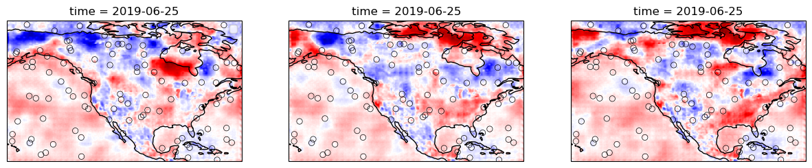
The checkerboard artefacts in the samples above correspond to the subsampled grid of AR sample target locations. This could be alleviated by training the model for longer and with more examples of larger/denser context sets.