TaskLoader

The TaskLoader generates Task objects for training, testing, and inference with DeepSensor models. The TaskLoader can generate Tasks for different kinds of predictions, such as: spatial interpolation, forecasting, downscaling, or some combination of these. It achieves this by temporally slicing spatiotemporal data and then providing a suite of spatial sampling methods for generating context and target sets from the temporal slices.

Mastering DeepSensor requires a good understanding of all the ways you can initialise and call a TaskLoader for a wide range of data fusion applications. The TaskLoader is best understood through examples, which we will see in this page. Let’s import the TaskLoader class and get started.

Show code cell content Hide code cell content

import logging

logging.captureWarnings(True)

import deepsensor.torch
from deepsensor.data import DataProcessor
from deepsensor.data.sources import get_ghcnd_station_data, get_era5_reanalysis_data, get_earthenv_auxiliary_data, get_gldas_land_mask

import matplotlib.pyplot as plt

# Using the same settings allows use to use pre-downloaded cached data
data_range = ("2016-06-25", "2016-06-30")
extent = "europe"
station_var_IDs = ["TAVG", "PRCP"]
era5_var_IDs = ["2m_temperature", "10m_u_component_of_wind", "10m_v_component_of_wind"]
auxiliary_var_IDs = ["elevation", "tpi"]
cache_dir = "../../.datacache"

station_raw_df = get_ghcnd_station_data(station_var_IDs, extent, date_range=data_range, cache=True, cache_dir=cache_dir)
era5_raw_ds = get_era5_reanalysis_data(era5_var_IDs, extent, date_range=data_range, cache=True, cache_dir=cache_dir)
auxiliary_raw_ds = get_earthenv_auxiliary_data(auxiliary_var_IDs, extent, "10KM", cache=True, cache_dir=cache_dir)
land_mask_raw_ds = get_gldas_land_mask(extent, cache=True, cache_dir=cache_dir)

data_processor = DataProcessor(x1_name="lat", x2_name="lon")
era5_ds = data_processor(era5_raw_ds)
aux_ds, land_mask_ds = data_processor([auxiliary_raw_ds, land_mask_raw_ds], method="min_max")
station_df = data_processor(station_raw_df)

from deepsensor.data import TaskLoader

Initialising a TaskLoader

A TaskLoader is initialised with list of context and target variables. These variables can either be xarray or pandas objects, and are assumed to have been standardised by a DataProcessor.

We will use the normalised station and reanalysis data from the previous DataProcessor page.

task_loader = TaskLoader(
    context=[era5_ds, land_mask_ds],
    target=station_df,
    aux_at_targets=aux_ds,
)
print(task_loader)

TaskLoader(2 context sets, 1 target sets)
Context variable IDs: (('2m_temperature', '10m_u_component_of_wind', '10m_v_component_of_wind'), ('GLDAS_mask',))
Target variable IDs: (('PRCP', 'TAVG'),)
Auxiliary-at-target variable IDs: ('elevation', 'tpi')

Calling a TaskLoader

The TaskLoader is called with a timestamp and single entries or lists of entries for the context_sampling and target_sampling arguments. These arguments can either be single entries (applying the same sampling strategy to each context/target set) or a list of entries equal to the number of context/target sets (applying different sampling strategies to each context/target set).

For an up-to-date list of the available sampling strategies and what they do, see the TaskLoader.task_generation documentation.

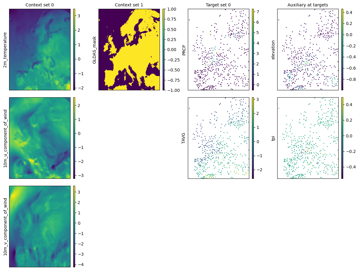
task = task_loader("2016-06-25", context_sampling="all", target_sampling="all")
print(task)

time: 2016-06-25 00:00:00
ops: []
X_c: [((1, 141), (1, 221)), ((1, 140), (1, 220))]
Y_c: [(3, 141, 221), (1, 140, 220)]
X_t: [(2, 519)]
Y_t: [(2, 519)]
Y_t_aux: (2, 519)

fig = deepsensor.plot.task(task, task_loader)
plt.show()

TaskLoader tour

Now that we’ve got the basics of the TaskLoader init and call signatures, let’s see some concrete examples of to generate Task objects for spatial interpolation, forecasting, downscaling, and gap-filling.

Spatial interpolation

Spatial interpolation tasks can be generated either from:

• gridded xarray data, by randomly sampling points from the grid, or

• pointwise pandas data, by randomly splitting the data into context and target sets.

Interpolating gridded xarray data

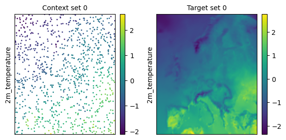
Randomly sampling a float fraction of points

task_loader = TaskLoader(context=era5_ds["2m_temperature"], target=era5_ds["2m_temperature"])
task = task_loader("2016-06-28", context_sampling=0.03, target_sampling="all")
print(task)

time: 2016-06-28 00:00:00
ops: []
X_c: [(2, 934)]
Y_c: [(1, 934)]
X_t: [((1, 141), (1, 221))]
Y_t: [(1, 141, 221)]

deepsensor.plot.task(task, task_loader)
plt.show()

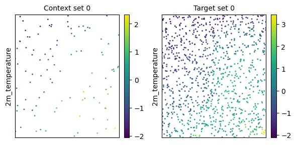
Randomly sampling a int number of points

task = task_loader("2016-06-25", context_sampling=100, target_sampling=1000)
print(task)

time: 2016-06-25 00:00:00
ops: []
X_c: [(2, 100)]
Y_c: [(1, 100)]
X_t: [(2, 1000)]
Y_t: [(1, 1000)]

deepsensor.plot.task(task, task_loader)
plt.show()

Interpolating pointwise pandas data

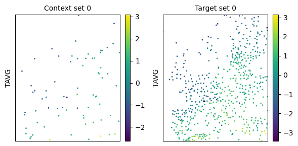
task_loader = TaskLoader(context=station_df["TAVG"], target=station_df["TAVG"], links=[(0, 0)])

task = task_loader("2016-06-25", context_sampling="split", target_sampling="split", split_frac=0.1)
print(task)

time: 2016-06-25 00:00:00
ops: []
X_c: [(2, 72)]
Y_c: [(1, 72)]
X_t: [(2, 592)]
Y_t: [(1, 592)]

deepsensor.plot.task(task, task_loader)
plt.show()

Forecasting

Using the context_delta_t and/or target_delta_t arguments, we can generate Tasks for forecasting. The values of context_delta_t and target_delta_t are time differences relative to the time slice passed to the TaskLoader (which may be considered as an ‘initialisation time’). The units of these time detlas are determined by the time_freq argument, which defaults to "D" (days).

task_loader = TaskLoader(
    context=[era5_ds["2m_temperature"],] * 3,
    context_delta_t=[-1, -2, 0],
    target=era5_ds["2m_temperature"],
    target_delta_t=1,
    time_freq="D",  # daily frequency (the default)
)
print(task_loader)

TaskLoader(3 context sets, 1 target sets)
Context variable IDs: (('2m_temperature',), ('2m_temperature',), ('2m_temperature',))
Target variable IDs: (('2m_temperature',),)

task = task_loader("2016-06-27", context_sampling="all", target_sampling="all")
print(task)

time: 2016-06-27 00:00:00
ops: []
X_c: [((1, 141), (1, 221)), ((1, 141), (1, 221)), ((1, 141), (1, 221))]
Y_c: [(1, 141, 221), (1, 141, 221), (1, 141, 221)]
X_t: [((1, 141), (1, 221))]
Y_t: [(1, 141, 221)]

deepsensor.plot.task(task, task_loader)
plt.show()

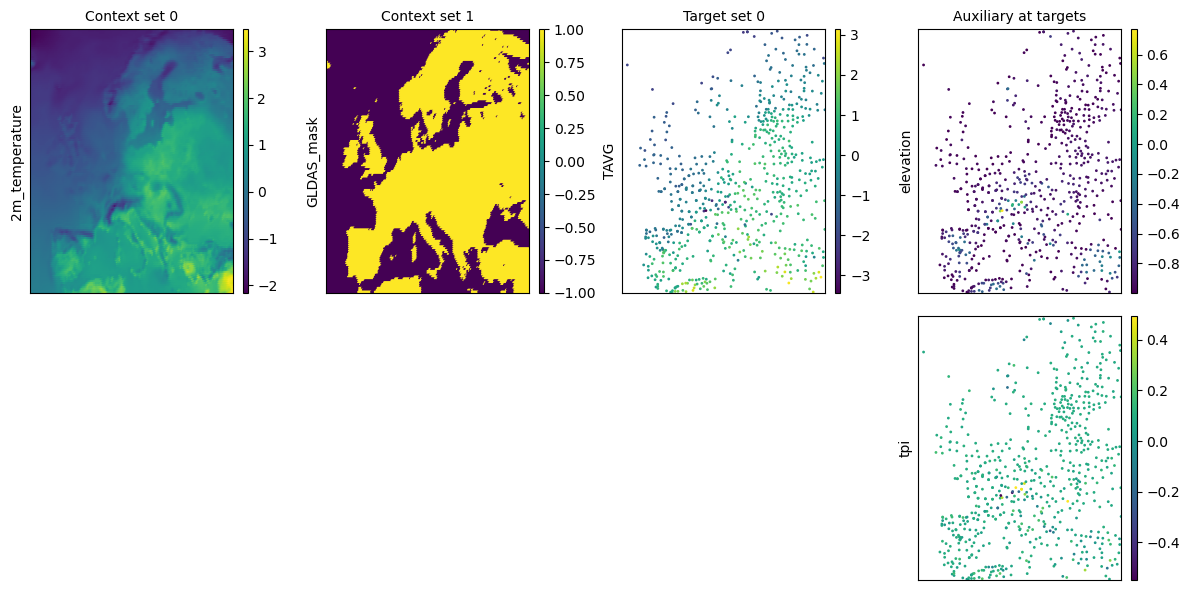
Downscaling

In statistical downscaling, the goal is often to learn a mapping from a coarse gridded data set (e.g. reanalysis data) to localised observations (e.g. weather station data). A downscaling TaskLoader can be instantiated by passing the coarse gridded variable in the context list and station observations in the target list.

Optionally, we can also pass a high-resolution auxiliary xarray variable (e.g. local topgraphic information) via the aux_at_targets argument. When calling the TaskLoader, the aux_at_targets variable will be interpolated at the target locations and added to the Task as the "Y_t_aux" entry. The "Y_t_aux" data can be modelled differently from the context data, for example, by using a pointwise MLP rather than a convolutional neural network.

Note

The TaskLoader also permits an aux_at_contexts argument for passing high-resolution auxiliary variables at off-grid context locations. For brevity, we will not demonstrate this here.

Hypothetically, with the right auxiliary information and enough data, a model can distinguish between an observation from the top of a mountain vs a valley vs a city vs a field.

task_loader = TaskLoader(
    context=[era5_ds["2m_temperature"], land_mask_ds],
    target=station_df["TAVG"],
    aux_at_targets=aux_ds,
)
print(task_loader)

TaskLoader(2 context sets, 1 target sets)
Context variable IDs: (('2m_temperature',), ('GLDAS_mask',))
Target variable IDs: (('TAVG',),)
Auxiliary-at-target variable IDs: ('elevation', 'tpi')

task = task_loader("2016-06-25", context_sampling="all", target_sampling="all")
print(task)

time: 2016-06-25 00:00:00
ops: []
X_c: [((1, 141), (1, 221)), ((1, 140), (1, 220))]
Y_c: [(1, 141, 221), (1, 140, 220)]
X_t: [(2, 664)]
Y_t: [(1, 664)]
Y_t_aux: (2, 664)

deepsensor.plot.task(task, task_loader)
plt.show()

Gap-filling

The TaskLoader can be used to generate training Tasks for filling missing data gaps in an xarray object.

Let’s generate some fake missing data in the normalised era5_ds object by setting all normalised temperature values below -0.75 to NaN. In practice, these may be missing due to cloud coverage, satellite orbit gaps, sensor issues, or other reasons.

era5_gappy_ds = era5_ds["2m_temperature"].where(era5_ds["2m_temperature"] > -0.75)
fig = era5_gappy_ds.plot(col="time", col_wrap=6, center=False)
plt.show()

If we pass the "gapfill" argument to the context_sampling and target_sampling arguments, the TaskLoader does the following:

• randomly samples a missing data mask from another time slice,

• adds this new mask to the context set (increasing the amount of missing data in the context set),

• the context points which were just removed by the new mask become the target set.

This may produce NaNs in the target set due to overlap between the original mask and new mask. To remove these NaNs, use the Task.remove_context_nans and Task.remove_target_nans methods.

task_loader = TaskLoader(context=era5_gappy_ds, target=era5_gappy_ds, links=[(0, 0)])
task = task_loader("2016-06-25", context_sampling="gapfill", target_sampling="gapfill")
print(task.remove_context_nans().remove_target_nans())

time: 2016-06-25 00:00:00
ops: ['context_nans_removed', 'target_nans_removed']
X_c: [(2, 22491)]
Y_c: [(1, 22491)]
X_t: [(2, 867)]
Y_t: [(1, 867)]

deepsensor.plot.task(task, task_loader, figsize=4)
plt.show()

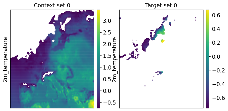
The spatial characteristics of the missing data in the context set appear realistic and will be similar to what the model will see when attempting to fill real missing data gaps.

Once a model is trained with Tasks generated with the "gapfill" strategy, the model can be used to fill real missing data by passing "all" for context_sampling.

Caution

Recall that we generated missing data by masking any normalised temperature values below -0.75 to NaN. This means that the true missing data is not representative of the observed data; the distribution of observed data is very different to the distribution of missing data. A model trained with the TaskLoader "gapfill" strategy will never see values below -0.75 and therefore its predictions will be heavily biased.

This is an extreme example, but the same effect can occur in real data sets. For example, if missing data comes from clouds and the target variable is temperature, a model trained with the "gapfill" strategy will not learn the effect of clouds on temperature.

Combinations of data fusion tasks

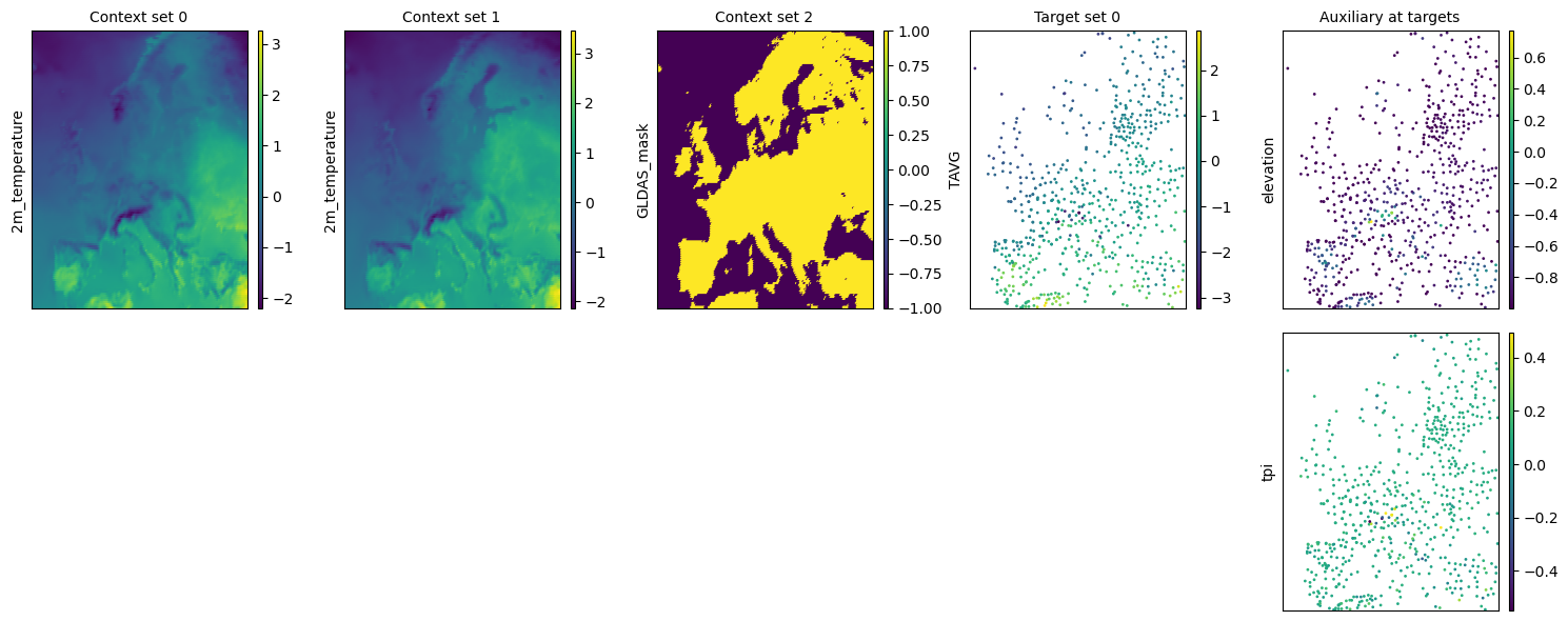
Real applications may involve a combination of the above data fusion tasks. The flexibility of the TaskLoader makes it easy to generate Tasks for diverse data fusion problems. Here’s a concrete example combining forecasting with downscaling, using the past two days of ERA5 data to forecast the next day of station observations, leveraging high-resolution auxiliary data.

task_loader = TaskLoader(
    context=[era5_ds["2m_temperature"], era5_ds["2m_temperature"], land_mask_ds],
    context_delta_t=[-1, -2, 0],
    target=station_df["TAVG"],
    target_delta_t=1,
    aux_at_targets=aux_ds,
)
print(task_loader)

TaskLoader(3 context sets, 1 target sets)
Context variable IDs: (('2m_temperature',), ('2m_temperature',), ('GLDAS_mask',))
Target variable IDs: (('TAVG',),)
Auxiliary-at-target variable IDs: ('elevation', 'tpi')

task = task_loader("2016-06-28", context_sampling="all", target_sampling="all")
print(task)

time: 2016-06-28 00:00:00
ops: []
X_c: [((1, 141), (1, 221)), ((1, 141), (1, 221)), ((1, 140), (1, 220))]
Y_c: [(1, 141, 221), (1, 141, 221), (1, 140, 220)]
X_t: [(2, 667)]
Y_t: [(1, 667)]
Y_t_aux: (2, 667)

deepsensor.plot.task(task, task_loader)
plt.show()

Controlling randomness in the TaskLoader

There are two additional arguments in the TaskLoader call method for controlling randomness:

• datewise_deterministic: If True, the same random seed will be used for a particlar date. Useful for, say, generating a reproducible validation set which is the same between Python sessions.

• seed_override: If not None, this seed will be used instead of the default seed.

Saving and loading a TaskLoader

You can save the TaskLoader object to a file using the .save method.

Note

Currently, saving a TaskLoader is only supported it it has been initialised with str paths to NetCDF or CSV files, allowing the TaskLoader to be represented with a configuration file which can then be saved and loaded. It would be useful to be able to save TaskLoaders initialised with xarray or pandas objects by saving the objects to NetCDF or CSV files under the hood. There is an issue open about this.

data_fpath = "tmp.nc"
era5_ds.to_netcdf(data_fpath)

task_loader = TaskLoader(context=data_fpath, target=data_fpath)
print(task_loader)

TaskLoader(1 context sets, 1 target sets)
Context variable IDs: (('2m_temperature', '10m_u_component_of_wind', '10m_v_component_of_wind'),)
Target variable IDs: (('2m_temperature', '10m_u_component_of_wind', '10m_v_component_of_wind'),)

task_loader.save("tmp/")

task_loader_loaded = TaskLoader("tmp/")
print(task_loader_loaded)

TaskLoader(1 context sets, 1 target sets)
Context variable IDs: (('2m_temperature', '10m_u_component_of_wind', '10m_v_component_of_wind'),)
Target variable IDs: (('2m_temperature', '10m_u_component_of_wind', '10m_v_component_of_wind'),)

import os
import shutil
os.remove(data_fpath)
shutil.rmtree("tmp/")