Quickstart

AutoEmulate’s goal is to make it easy to create an emulator for your simulation. Here’s the basic workflow:

import numpy as np
import random
import torch
from autoemulate.compare import AutoEmulate
from autoemulate.experimental_design import LatinHypercube
from autoemulate.simulations.projectile import simulate_projectile

seed = 43 
np.random.seed(seed)
random.seed(seed)
_ = torch.manual_seed(seed)

Design of Experiments

Before we build an emulator or surrogate model, we need to get a set of input/output pairs from the simulation. This is called the Design of Experiments (DoE) and is currently not a key part of AutoEmulate, as this step is tricky to automate and will run on more complex compute infrastructure for expensive simulations. There are lots of sampling techniques, but here we are using Latin Hypercube Sampling.

Below, simulate_projectile is a simulation for a projectil motion with drag (see here for details). It takes two inputs, the drag coefficient (on a log scale) and the velocity and outputs the distance the projectile travelled. We sample 100 sets of inputs X using a Latin Hypercube Sampler and run the simulator for those inputs to get the outputs y.

# sample from a simulation
lhd = LatinHypercube([(-5., 1.), (0., 1000.)]) # (upper, lower) bounds for each parameter
X = lhd.sample(100)
y = np.array([simulate_projectile(x) for x in X])
X.shape, y.shape

((100, 2), (100,))

Comparing emulators

This is the core of AutoEmulate. With a set of inputs / outputs, we can run a full machine learning pipeline, including data processing, model fitting, model selection and potentially hyperparameter optimisation in just a few lines of code. First, we initialise an AutoEmulate object. Then, we run setup(X, y), providing the simulation inputs and outputs. Lastly, compare() will fit a range of different models to the data and evaluate them using cross-validation, returning the best emulator.

# compare emulator models
ae = AutoEmulate()
ae.setup(X, y)
ae.compare()

AutoEmulate is set up with the following settings:

	Values
Simulation input shape (X)	(100, 2)
Simulation output shape (y)	(100,)
Proportion of data for testing (test_set_size)	0.2
Scale input data (scale)	True
Scaler (scaler)	StandardScaler
Scale output data (scale_output)	True
Scaler output (scaler_output)	StandardScaler
Do hyperparameter search (param_search)	False
Reduce input dimensionality (reduce_dim)	False
Reduce output dimensionality (reduce_dim_output)	False
Cross validator (cross_validator)	KFold
Parallel jobs (n_jobs)	1

InputOutputPipeline(regressor=Pipeline(steps=[('scaler', StandardScaler()),
                                              ('model', GaussianProcess())]),
                    transformer=Pipeline(steps=[('scaler_output',
                                                 StandardScaler())]))

In a Jupyter environment, please rerun this cell to show the HTML representation or trust the notebook.
On GitHub, the HTML representation is unable to render, please try loading this page with nbviewer.org.

We can have a look at the average cross-validation results for each model:

ae.summarise_cv()

	preprocessing	model	short	fold	rmse	r2
0	None	GaussianProcess	gp	3	109.516883	0.999684
1	None	RadialBasisFunctions	rbf	3	149.299730	0.999412
2	None	GaussianProcess	gp	4	313.779301	0.997543
3	None	RadialBasisFunctions	rbf	4	367.621737	0.996627
4	None	GaussianProcess	gp	1	272.691380	0.994329
5	None	GaussianProcess	gp	2	578.136242	0.994281
6	None	GaussianProcess	gp	0	1325.387105	0.989420
7	None	RadialBasisFunctions	rbf	2	943.636906	0.984764
8	None	GradientBoosting	gb	3	1027.184437	0.972178
9	None	RandomForest	rf	3	1080.518273	0.969213
10	None	RadialBasisFunctions	rbf	1	642.555947	0.968513
11	None	GradientBoosting	gb	1	659.140181	0.966866
12	None	SupportVectorMachines	svm	1	874.875848	0.941627
13	None	ConditionalNeuralProcess	cnp	2	1894.547971	0.938585
14	None	RadialBasisFunctions	rbf	0	3573.354920	0.923096
15	None	SupportVectorMachines	svm	4	1930.202881	0.907027
16	None	SupportVectorMachines	svm	3	2092.453397	0.884546
17	None	SecondOrderPolynomial	sop	3	2400.916075	0.847997
18	None	SecondOrderPolynomial	sop	4	2550.814541	0.837629
19	None	ConditionalNeuralProcess	cnp	3	2655.422293	0.814063
20	None	RandomForest	rf	2	3299.003867	0.813778
21	None	SupportVectorMachines	svm	2	3400.688299	0.802122
22	None	GradientBoosting	gb	2	3476.513111	0.793199
23	None	ConditionalNeuralProcess	cnp	1	1747.060865	0.767227
24	None	GradientBoosting	gb	0	6512.637952	0.744549
25	None	LightGBM	lgbm	3	3119.478550	0.743397
26	None	SecondOrderPolynomial	sop	0	7255.304581	0.682967
27	None	RandomForest	rf	0	7389.997800	0.671086
28	None	ConditionalNeuralProcess	cnp	0	7970.759899	0.617357
29	None	RandomForest	rf	1	2283.013567	0.602504
30	None	RandomForest	rf	4	4062.929829	0.588064
31	None	LightGBM	lgbm	4	4087.601934	0.583046
32	None	SupportVectorMachines	svm	0	8904.240487	0.522484
33	None	ConditionalNeuralProcess	cnp	4	4445.580411	0.506818
34	None	SecondOrderPolynomial	sop	2	5427.528875	0.495956
35	None	LightGBM	lgbm	2	5577.039563	0.467804
36	None	LightGBM	lgbm	0	9746.822347	0.427837
37	None	GradientBoosting	gb	4	5043.883814	0.365136
38	None	SecondOrderPolynomial	sop	1	3122.018792	0.256661
39	None	LightGBM	lgbm	1	4370.289332	-0.456587

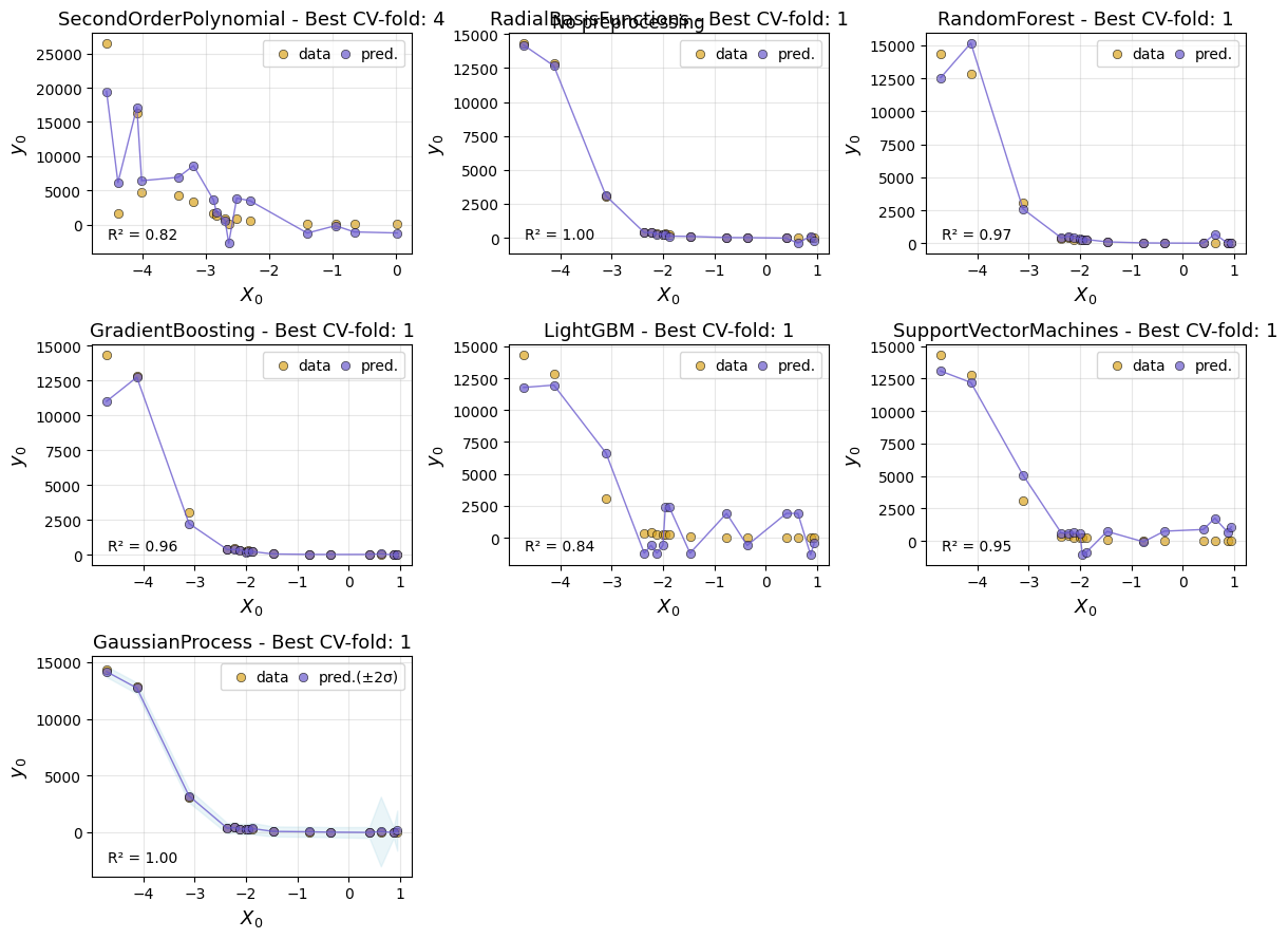
And create plots comparing the models:

ae.plot_cv()

Using best preprocessing method: None

No preprocessing was applied (using raw target values)

Evaluating on the test set

AutoEmulate has already split the data into a training set and a test set. After looking at the cross-validation results, we can retrieve a fitted emulator and evaluate it on the test set. The GP predicts well on unseen data.

gp = ae.get_model("GaussianProcess")
ae.evaluate(gp)

	model	short	preprocessing	rmse	r2
0	GaussianProcess	gp	None	100.2043	0.9997

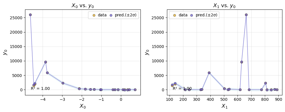
But it’s always useful to plot the predictions too.

ae.plot_eval(gp, input_index=[0, 1])

Refitting the emulator

Before applying the emulator, we refit it on the entire dataset, including training and test set. This is done with the refit() method.

gp_final = ae.refit(gp)

Predictions

We can use the best model to make predictions for new inputs. Emulators in AutoEmulate are scikit-learn estimators, so we can use the predict method to make predictions.

gp_final.predict(X[:10])

array([ 5.92802989e+03,  8.09320459e+03,  1.64314306e+04,  8.03658722e+03,
        1.02199569e+02, -4.13382376e+00,  6.15225062e+00,  5.94727985e+01,
        1.08353372e+04,  7.00209722e+00])

Saving / loading models

Lastly, we can save and load an emulator. To load, we need an initialised AutoEmulate object. This will ensure that the environment in which the model was saved is similar to the environment in which it is loaded.

# # save & load best emulator
# ae.save(gp_final, "gp_final")
# emulator = ae.load("gp_final")