Reduced-dimension Emulator: Reaction-Diffusion example#
Overview#
In this example, we aim to create an emulator to generate solutions to a 2D parameterized reaction-diffusion problem governed by the following partial differential equations:
where:
\( u \) and \( v \) are the concentrations of two species,
\( \beta \) and \( d \) control the reaction and diffusion terms.
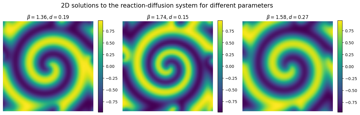
This system exhibits complex spatio-temporal dynamics such as spiral waves.
import numpy as np
import pandas as pd
import matplotlib.pyplot as plt
import autoemulate as ae
from tqdm import tqdm
import os

from autoemulate.experimental_design import LatinHypercube
from autoemulate.simulations.reaction_diffusion import simulate_reaction_diffusion
from autoemulate.compare import AutoEmulate

save = False
train = False
1) Data generation#
Data are computed using a numerical simulator using Fourier spectral method. The simulator takes two inputs: the reaction parameter \(\beta\) and the diffusion parameter \(d\).
We sample 50 sets of inputs X using Latin Hypercube sampling and run the simulator for those inputs to get the solutions Y.
n = 50

# Reaction-diffusion parameters
beta = (1., 2.) # lower and upper bounds for the reaction coefficient
d = (0.05, 0.3) # lower and upper bounds for the diffusion coefficient
lhd = LatinHypercube([beta, d])
n_samples = 50
X = lhd.sample(n_samples)

data_folder = "../data/reaction_diffusion"
if not os.path.exists(data_folder):
    os.makedirs(data_folder)
X_file = os.path.join(data_folder, "X.csv")
Y_file = os.path.join(data_folder, "Y.csv")

if train:
    # Run the simulator to generate data
    U, V = zip(*[simulate_reaction_diffusion(x, n=n, T=10) for x in tqdm(X)])
    U = np.stack(U)
    V = np.stack(V)

    # Let's consider as output the concentration of the specie U
    Y = U.reshape(n_samples, -1)

    if save:
        # Save the data
        pd.DataFrame(X).to_csv(X_file, index=False)
        pd.DataFrame(Y).to_csv(Y_file, index=False)
else:
    # Load the data
    X = pd.read_csv(X_file).values
    Y = pd.read_csv(Y_file).values

print(f"shapes: input X: {X.shape}, output Y: {Y.shape}\n")
shapes: input X: (50, 2), output Y: (50, 2500)
X and Y are matrices where each row represents one run of the simulation. In the input matrix X the two columuns indicates the input parameters (reaction \(\beta\) and diffusion \(d\) parameters, respetively).
In the output matrix Y each column indicates a spatial location where the solution (i.e. the concentration of \(u\) at final time \(T=10\)) is computed.
We consider a 2D spatial grid of \(50\times 50\) points, therefore each row of Y corresponds to a 2500-dimensional vector!
Let’s now plot the simulated data to see how the reaction-diffusion pattern looks like.
plt.figure(figsize=(15,4.5))
for param in range(3):
  plt.subplot(1,3,1+param)
  plt.imshow(Y[param].reshape(n,n), interpolation='bilinear')
  plt.axis('off')
  plt.xlabel('x', fontsize=12)
  plt.ylabel('y')
  plt.title(r'$\beta = {:.2f}, d = {:.2f}$'.format(X[param][0], X[param][1]), fontsize=12)
  plt.colorbar(fraction=0.046)
plt.suptitle('2D solutions to the reaction-diffusion system for different parameters', fontsize=15)
plt.show()
2) Reduced-dimension Emulator#
The numerical simulator is computationally expensive to run, thus we aim to replace it with a fast emulator. As output we aim to emulate is the full spatial fields of the concentration of \(u\) which is high-dimensional, we employ dimensionality reduction techniques to create a faster and more efficient emulator.
You can do so by selecting reduce_dim_output=True and indicate in a dictionary preprocessing_methods, which dimensionality reducer you want to use among
"PCA": Principal Component Analysis,"VAE": Variational Autoencoder,
which will be trained together with the emulator.
More details about the dimensionality reudcers can be provided as params, such as reduced_dim to select how many latents varaibles we want to consider (e.g., if reduced_dim = 8, we compress 2500-dimensional data into a 8-dimensional variables), or hyperparameters (learning rate, batch_size, etc.) for deep learning methhods.
em = AutoEmulate()

preprocessing_methods = [{"name": "PCA", "params": {"reduced_dim": 8}},
                         {"name": "PCA", "params": {"reduced_dim": 16}},
                         {"name": "VAE", "params": {"reduced_dim": 8}},
                         {"name": "VAE", "params": {"reduced_dim": 16, "learning_rate" : 1e-4, "batch_size" : 16, "epochs": 5000, "beta": 1e-4}}]

em.setup(X, Y, scale_output=True, reduce_dim_output=True, preprocessing_methods=preprocessing_methods)
AutoEmulate is set up with the following settings:
| Values | |
|---|---|
| Simulation input shape (X) | (50, 2) |
| Simulation output shape (y) | (50, 2500) |
| Proportion of data for testing (test_set_size) | 0.2 |
| Scale input data (scale) | True |
| Scaler (scaler) | StandardScaler |
| Scale output data (scale_output) | True |
| Scaler output (scaler_output) | StandardScaler |
| Do hyperparameter search (param_search) | False |
| Reduce input dimensionality (reduce_dim) | False |
| Reduce output dimensionality (reduce_dim_output) | True |
| Dimensionality output reduction methods (dim_reducer_output) | PCA, VAE |
| Cross validator (cross_validator) | KFold |
| Parallel jobs (n_jobs) | 1 |
AutoEmulate automatically selects the best combination of dimesnionality reducer and model, just by running .compare().
best_model = em.compare()
best_model
InputOutputPipeline(regressor=Pipeline(steps=[('scaler', StandardScaler()),
                                              ('model', GaussianProcess())]),
                    transformer=Pipeline(steps=[('scaler_output',
                                                 StandardScaler()),
                                                ('dim_reducer_output',
                                                 PCA(n_components=16))]))
In a Jupyter environment, please rerun this cell to show the HTML representation or trust the notebook. On GitHub, the HTML representation is unable to render, please try loading this page with nbviewer.org.
InputOutputPipeline(regressor=Pipeline(steps=[('scaler', StandardScaler()),
                                              ('model', GaussianProcess())]),
                    transformer=Pipeline(steps=[('scaler_output',
                                                 StandardScaler()),
                                                ('dim_reducer_output',
PCA(n_components=16))]))Pipeline(steps=[('scaler', StandardScaler()), ('model', GaussianProcess())])StandardScaler()
GaussianProcess()
Pipeline(steps=[('scaler_output', StandardScaler()),
('dim_reducer_output', PCA(n_components=16))])StandardScaler()
PCA(n_components=16)
3) Summarising cross-validation results#
We can look at the cross-validation results to see which model provides the best emulator.
em.summarise_cv()
| preprocessing | model | short | fold | rmse | r2 | |
|---|---|---|---|---|---|---|
| 0 | PCA | GaussianProcess | gp | 4 | 0.042386 | 0.993151 |
| 1 | PCA | GaussianProcess | gp | 1 | 0.050584 | 0.989707 |
| 2 | PCA | GaussianProcess | gp | 2 | 0.050794 | 0.988663 |
| 3 | PCA | GaussianProcess | gp | 0 | 0.079627 | 0.982349 |
| 4 | PCA | GaussianProcess | gp | 3 | 0.091489 | 0.970318 |
| ... | ... | ... | ... | ... | ... | ... |
| 65 | VAE | LightGBM | lgbm | 3 | 0.649900 | -0.167198 |
| 66 | VAE | SecondOrderPolynomial | sop | 3 | 0.642020 | -0.176219 |
| 67 | VAE | LightGBM | lgbm | 4 | 0.653343 | -0.219246 |
| 68 | VAE | LightGBM | lgbm | 2 | 0.656918 | -0.390903 |
| 69 | VAE | SecondOrderPolynomial | sop | 1 | 0.693792 | -0.519905 |
70 rows × 6 columns
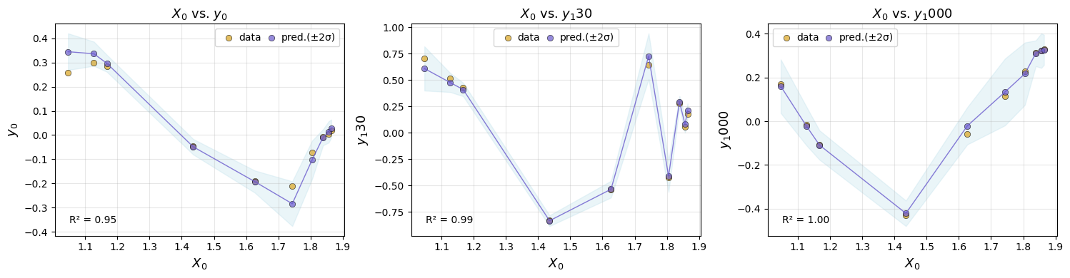
We can select the best performing emulator model (in this case GaussianProcess) and see how it performs on the test-set, which AutoEmulate automatically sets aside.
We can plot the test-set performance for chosen emulator.
gp = em.get_model('GaussianProcess')
em.evaluate(gp)
| model | short | preprocessing | rmse | r2 | |
|---|---|---|---|---|---|
| 0 | GaussianProcess | gp | PCA | 0.0631 | 0.9851 |
em.plot_eval(gp, input_index=[0], output_index=[0,130,1000])
4) Refitting the model on the full dataset#
AutoEmulate splits the dataset into a training and holdout set. All cross-validation, parameter optimisation and model selection is done on the training set. After we selected a best emulator model, we can refit it on the full traiing dataset.
gp_final = em.refit(gp)
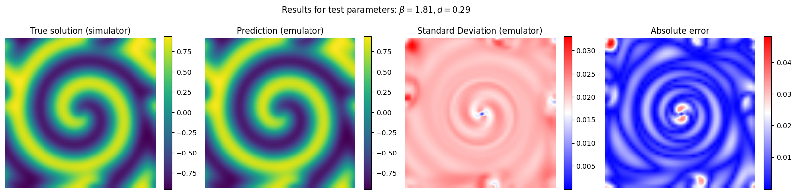
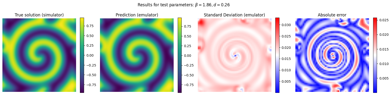
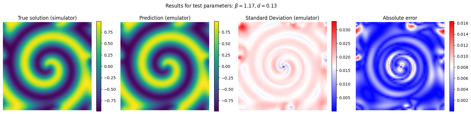
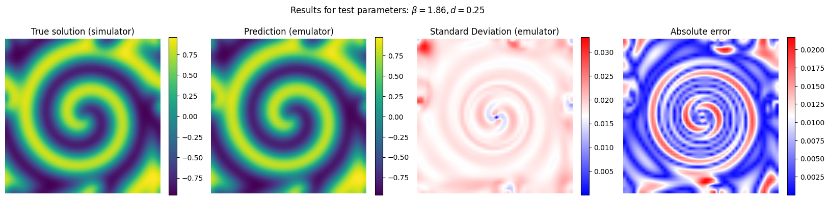
5) Predict on the test set#
Now we run the emulator for unseen combinations of reaction and diffusion parameter and we compare its performance with respect to the reference (simulator)
y_pred, y_std_pred  = gp_final.predict(X[em.test_idxs], return_std = True)
y_true = Y[em.test_idxs]
# Plot the results for some unseen (test) parameter instances
params_test = [0,1,2,3]

for param_test in params_test:
  plt.figure(figsize=(20,4.5))
  plt.subplot(1,4,1)
  plt.imshow(y_true[param_test].reshape(n,n), interpolation='bilinear')
  plt.axis('off')
  plt.xlabel('x', fontsize=12)
  plt.ylabel('y')
  plt.title('True solution (simulator)', fontsize=12)
  plt.colorbar(fraction=0.046)

  plt.subplot(1,4,2)
  plt.imshow(y_pred[param_test].reshape(n,n), interpolation='bilinear')
  plt.axis('off')
  plt.xlabel('x', fontsize=12)
  plt.ylabel('y')
  plt.title('Prediction (emulator)', fontsize=12)
  plt.colorbar(fraction=0.046)

  plt.subplot(1,4,3)
  plt.imshow(y_std_pred[param_test].reshape(n,n), cmap = 'bwr', interpolation='bilinear', vmax = np.max(y_std_pred[params_test]))
  plt.axis('off')
  plt.xlabel('x', fontsize=12)
  plt.ylabel('y')
  plt.title('Standard Deviation (emulator)', fontsize=12)
  plt.colorbar(fraction=0.046)

  plt.subplot(1,4,4)
  plt.imshow(np.abs(y_pred[param_test] - y_true[param_test]).reshape(n,n), cmap = 'bwr', interpolation='bilinear')
  plt.axis('off')
  plt.xlabel('x', fontsize=12)
  plt.ylabel('y')
  plt.title('Absolute error', fontsize=12)
  plt.colorbar(fraction=0.046)

  plt.suptitle(r'Results for test parameters: $\beta = {:.2f}, d = {:.2f}$'.format(X[em.test_idxs][param_test][0], X[em.test_idxs][param_test][1]), fontsize=12)
  plt.show()