Scaling Sensitivity Analysis with Emulation

In this tutorial we demonstrate how AutoEmulate can facilitate finding the best emulator for the simulation of fluid flow in a cardiovascular system.

By the end of this tutorial:

• Participants will learn how to use Autoemulate for the emulation of a real-world simulation in an end-to-end pipeline.

• Participants will learn how to explore the relationship between underlying cardiac health parameters and non-invasive measures using synthetic data, with a focus on how these insights can improve understanding and estimation of key cardiovascular dynamics

The Problem

In the field of cardiovascular modeling, capturing the dynamics of blood flow and the associated pressures and volumes within the vascular system is crucial for understanding heart function and disease. Physics-based models that accurately represent these dynamics often require significant computational resources, making them challenging to apply in large-scale or real-time scenarios. Emulation techniques provide a way to achieve high-fidelity simulations of the cardiovascular system, allowing for efficient and accurate analysis of key hemodynamic parameters.

Content

This tutorial includes:

1. Setting up a simulation : The system simulated is a tube with an input flow rate at any given time. The tube is divided to 10 compartments which allows for the study of the pressure and flow rate at various points in the tube.

2. Running the simulation for 60 sets of parameters sampled from the parameter space.

3. Using Autoemulate to find the best emulator fot this simulation

4. Assessing model accuracy, performing sensitivity analysis.

import os
import numpy as np
import pandas as pd
import matplotlib.pyplot as plt
from tqdm import tqdm
from autoemulate.compare import AutoEmulate
from sklearn.metrics import r2_score

from autoemulate.experimental_design import LatinHypercube
from autoemulate.simulations.flow_functions import FlowProblem

show_progress = False if os.getenv("JUPYTER_BOOK_BUILD", "false").lower() == "true" else True

Define your simulator

This simulator simulates a vessel divided to 10 compartments.

Parameters

The simulation parameters include :

1. R (Resistance): Represents the resistance to blood flow in blood vessels, akin to the hydraulic resistance caused by vessel diameter and blood viscosity (Analogous to electrical resistor).

2. L (Inductance): Represents the inertial effects of blood flow, capturing how blood resists changes in its velocity (Analogous to electrical inductor).

3. C (Capacitance): Represents the compliance or elasticity of blood vessels, primarily large arteries, which store and release blood volume with changes in pressure (Analogous to a capacitor).

Boundary conditions

1. Neumann boundary condition : Specifies the derivative of the variable at the boundary.

2. Dirichlet Boundary condition : Specifies the value of the variable directly at the boundary.

The setup

The input flow rate in each compartment is \(Q_i(t)\) for the \(i^{th}\) compartment and the output flow rate is \(Q_{i+1}(t)\).

\(Q_0(t) = \begin{cases} A \cdot \sin^2\left(\frac{\pi}{t_d} t\right), & \text{if } 0 \leq t < T, \\ 0, & \text{otherwise}. \end{cases}\)

Where:

• \(Q_0(t)\) is the input pulse function (flow rate) at time t

• A is the amplitude of the pulse

• \(t_d\) is the pulse duration.

fp = FlowProblem(ncycles=10, ncomp=10, amp=900.)
fp.generate_pulse_function()

Solve

Pressure in Each Compartment (\(P_i\)): This determines how the pressure in each compartment evolves over time, based on the inflow (\(Q_i(t)\)) and the outflow (\(Q_{i+1}(t)\)). where \(i\) is the number of compartment.

\(\frac{dP_i}{dt} = \frac{1}{C_n} \left( Q_i(t) - Q_{i+1}(t) \right)\) where, \(C_n = \frac{C}{n_\text{comp}}\)

Flow rate equation (\(Q_i\)): This governs how the flow in each compartment changes over time, depending on the pressures in the neighboring compartments and the resistance and inertance properties of each compartment.

\(\frac{dQ_i}{dt} = \frac{1}{L_n} \left( P_i - P_{10} - R_n Q_i(t) \right)\), where \(L_n = \frac{L}{n_\text{comp}}, \quad R_n = \frac{R}{n_\text{comp}}\)

fp.solve()

Plotting Pressure and flow rate

Here the pressure and flow rate have been plotted for all 10 compartments (the colour of the line fades for later compartments). As it is apaprent from the figure the peak pressure as well as the flow rate drops for the later compartments.

fig, ax = fp.plot_res()
plt.show()

Experimental Design

We set up the parameters for the simulation and their range. The range is set to the domain of interest for the problem we are solving. Furthermore, it is important to restrict the range to enhance the fitting of the model.

## specify valid parameter ranges
# Dictionary with parameters and their scaled ranges for the blood flow model
parameters_range = {
    'T': tuple(np.array([0.5, 1.5]) * 1.0),  # Cardiac cycle period (s)
    'td': tuple(np.array([0.8, 1.2]) * 0.2),  # Pulse duration (s)
    'amp': tuple(np.array([0.8, 1.2]) * 900.0),  # Amplitude (e.g., pressure or flow rate)
    'dt': tuple(np.array([0.5, 1.5]) * 0.001),  # Time step (s)
    'C': tuple(np.array([0.8, 1.2]) * 38.0),  # Compliance (unit varies based on context)
    'R': tuple(np.array([0.8, 1.2]) * 0.06),  # Resistance (unit varies based on context)
    'L': tuple(np.array([0.8, 1.2]) * 0.0017),  # Inductance (unit varies based on context)
    'R_o': tuple(np.array([0.8, 1.2]) * 0.025),  # Outflow resistance (unit varies based on context)
    'p_o': tuple(np.array([0.9, 1.1]) * 10.0)  # Initial pressure (unit varies based on context)
}

# Output the dictionary for verification

parameters_range

{'T': (0.5, 1.5),
 'td': (0.16000000000000003, 0.24),
 'amp': (720.0, 1080.0),
 'dt': (0.0005, 0.0015),
 'C': (30.400000000000002, 45.6),
 'R': (0.048, 0.072),
 'L': (0.00136, 0.0020399999999999997),
 'R_o': (0.020000000000000004, 0.03),
 'p_o': (9.0, 11.0)}

Sampling parameters

Secondly we sample the parameter space usning the Latin hypercube sampling (LHS) method.

Latin Hypercube Sampling (LHS) is a statistical method used for generating a sample of plausible values from a multidimensional distribution and guarantees that every sample is drawn from a different quantile of the underlying distribution. It is particularly effective for uncertainty quantification, sensitivity analysis, and simulation studies where the goal is to explore the behavior of a system or a model across a wide range of input parameter values.

## sample from parameter range

N_samples = 60
lhd = LatinHypercube(parameters_range.values())
sample_array = lhd.sample(N_samples)
sample_df    = pd.DataFrame(sample_array, columns=parameters_range.keys())  
print("Number of parameters", sample_df.shape[1], "Number of samples from each parameter", sample_df.shape[0])
sample_df.head()

Number of parameters 9 Number of samples from each parameter 60

	T	td	amp	dt	C	R	L	R_o	p_o
0	1.461289	0.215712	822.419671	0.000546	31.862459	0.065804	0.001812	0.029764	9.758126
1	1.372049	0.221633	1028.682521	0.000817	39.712955	0.057683	0.001821	0.028014	10.386695
2	0.865946	0.175274	1046.449330	0.000649	39.893196	0.051150	0.001915	0.021537	9.356704
3	0.831636	0.208146	874.279977	0.001003	30.891045	0.071650	0.001564	0.023347	10.687688
4	0.624389	0.161996	816.774962	0.000551	35.958400	0.062818	0.001577	0.025477	10.240238

Enforcing relationship between correlated parameters

The parameters are randomly sampled from the parameter space. However, some of the parameters are by nature correlated. For example in our simulation the duration of the pulse \(t_d\) is directly correlated with \(T\) which is the length of a full cycle. In this cell, we enforce the relationship between these two parameters. In otherwords scale \(t_d\) in accordance with the value of \(T\).

# enforce parameter relations (eg td <= T)
sample_df['td'] = sample_df.apply(lambda row: row['td']* row['T'], axis=1)

Simulate

Here we run the simulation which involves:
1- Generating the pulse functions.
2- Solving the differential equations.
3- Returning the pressure and flow rate in y for every set of parameters sampled (every row of sample_df data frame).

The full output of the simulation is quite large for fitting an emulator model. Therefore, it is standard practice to grab the most relavant information for training the emulator. Here we have chosen to train the emulator on the maximum pressure in each compartment. There are a variety of outputs that could be considered (max / min / average /mean / median / gradiant / PCA ).

# Fixed parameters: Number of compartments and cycles
ncomp = 10
ncycles = 10

# Function to run a simulation for a given set of parameters
def simulate(param_dict):
    fp = FlowProblem(ncycles=ncycles, ncomp=ncomp, **param_dict)
    fp.generate_pulse_function()
    fp.solve()
    return fp, fp.res.t, fp.res.y

Y = []
# Iterate over each sample of parameters
for index, row in tqdm(sample_df.iterrows(), total=len(sample_df), disable=show_progress):
    param_dict = row.to_dict() 
    fp, t, y = simulate(param_dict) 
    # extract peak pressure
    peak_pressure = y[:ncomp, :].max()
    Y.append(peak_pressure)

Emulate & Validate

Here we setup Autoemulate.

The models currently available for performing cross-validation are as follows:

• sop: SecondOrderPolynomial

• rbf: RadialBasisFunctions

• rf: RandomForest

• gb: GradientBoosting

• lgbm: LightGBM

• svm: SupportVectorMachines

• gp: GaussianProcess

• gpmt: GaussianProcessMT

• gps: GaussianProcessSklearn

• nns: NeuralNetSk

We have selected four of these models for cross-validation, feel free to explore more!

em = AutoEmulate()
parameter_names = list(parameters_range.keys())
em.setup(sample_df[parameter_names], Y, models = ['gp', 'svm','lgbm'])
best_model = em.compare()

AutoEmulate is set up with the following settings:

	Values
Simulation input shape (X)	(60, 9)
Simulation output shape (y)	(60,)
Proportion of data for testing (test_set_size)	0.2
Scale input data (scale)	True
Scaler (scaler)	StandardScaler
Scale output data (scale_output)	True
Scaler output (scaler_output)	StandardScaler
Do hyperparameter search (param_search)	False
Reduce input dimensionality (reduce_dim)	False
Reduce output dimensionality (reduce_dim_output)	False
Cross validator (cross_validator)	KFold
Parallel jobs (n_jobs)	1

em.summarise_cv()

	preprocessing	model	short	fold	rmse	r2
0	None	GaussianProcess	gp	3	7.261414	0.993317
1	None	GaussianProcess	gp	2	7.567520	0.992787
2	None	GaussianProcess	gp	4	10.248733	0.991203
3	None	GaussianProcess	gp	0	7.617236	0.990391
4	None	GaussianProcess	gp	1	5.569195	0.988490
5	None	SupportVectorMachines	svm	0	31.535972	0.835292
6	None	SupportVectorMachines	svm	1	21.985619	0.820625
7	None	SupportVectorMachines	svm	2	40.445935	0.793961
8	None	SupportVectorMachines	svm	4	55.638385	0.740733
9	None	SupportVectorMachines	svm	3	46.430346	0.726779
10	None	LightGBM	lgbm	2	89.123300	-0.000422
11	None	LightGBM	lgbm	0	77.973487	-0.006920
12	None	LightGBM	lgbm	1	52.106284	-0.007544
13	None	LightGBM	lgbm	3	89.253761	-0.009634
14	None	LightGBM	lgbm	4	110.019115	-0.013759

gp = em.get_model("GaussianProcess")
em.evaluate(gp)

	model	short	preprocessing	rmse	r2
0	GaussianProcess	gp	None	13.1617	0.9807

em.plot_eval(gp)

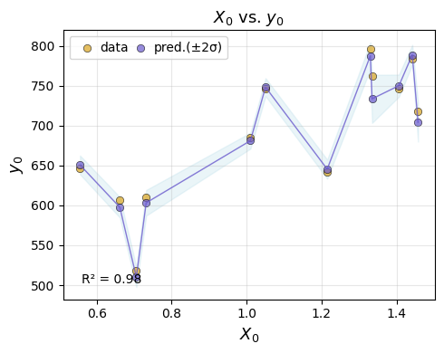
best_emulator = em.refit(gp)

Sensitivity Analysis

1. Define the problem by creating a dictionary which contains the names and the boundaries of the parameters

2. contribution of each parameter , importance of each parameter

   • S₁: First-order sensitivity index.

   • S₂: Second-order sensitivity index.

   • Sₜ: Total sensitivity index.

# Extract parameter names and bounds from the dictionary
parameter_names = list(parameters_range.keys())
parameter_bounds = list(parameters_range.values())

# Define the problem dictionary for Sobol sensitivity analysis
problem = {
    'num_vars': len(parameter_names),
    'names': parameter_names,
    'bounds': parameter_bounds
}

em.sensitivity_analysis(problem=problem)

	output	parameter	index	value	confidence
0	y1	T	S1	2.788484e-03	0.000234
1	y1	td	S1	1.886164e-02	0.001510
2	y1	amp	S1	8.897536e-01	0.052784
3	y1	dt	S1	9.171589e-05	0.000015
4	y1	C	S1	3.087203e-02	0.002608
5	y1	R	S1	5.425209e-02	0.004620
6	y1	L	S1	2.835864e-03	0.000256
7	y1	R_o	S1	1.980694e-04	0.000028
8	y1	p_o	S1	1.172785e-04	0.000018
0	y1	T	ST	3.217704e-03	0.004684
1	y1	td	ST	1.853837e-02	0.011843
2	y1	amp	ST	8.915814e-01	0.065410
3	y1	dt	ST	6.974099e-05	0.000959
4	y1	C	ST	3.035030e-02	0.014356
5	y1	R	ST	5.401306e-02	0.018120
6	y1	L	ST	2.589194e-03	0.005272
7	y1	R_o	ST	1.751505e-04	0.001463
8	y1	p_o	ST	-1.861986e-03	0.000855
0	y1	(T, td)	S2	-5.467348e-04	0.007053
1	y1	(T, amp)	S2	-6.566050e-04	0.009095
2	y1	(T, dt)	S2	-5.298052e-04	0.006939
3	y1	(T, C)	S2	-4.939709e-04	0.007050
4	y1	(T, R)	S2	-6.391547e-04	0.006951
5	y1	(T, L)	S2	-5.844973e-04	0.007051
6	y1	(T, R_o)	S2	-5.622995e-04	0.006906
7	y1	(T, p_o)	S2	-5.508073e-04	0.006941
8	y1	(td, amp)	S2	3.985405e-04	0.022118
9	y1	(td, dt)	S2	3.431409e-05	0.014411
10	y1	(td, C)	S2	1.335391e-04	0.014501
11	y1	(td, R)	S2	1.964116e-04	0.015096
12	y1	(td, L)	S2	1.644963e-05	0.014513
13	y1	(td, R_o)	S2	9.176998e-05	0.014429
14	y1	(td, p_o)	S2	1.551722e-05	0.014405
15	y1	(amp, dt)	S2	-1.328291e-04	0.080405
16	y1	(amp, C)	S2	1.398159e-04	0.081473
17	y1	(amp, R)	S2	-1.990180e-04	0.085640
18	y1	(amp, L)	S2	-7.041292e-05	0.080088
19	y1	(amp, R_o)	S2	-2.342571e-04	0.080054
20	y1	(amp, p_o)	S2	1.722009e-03	0.080165
21	y1	(dt, C)	S2	-3.068487e-05	0.001460
22	y1	(dt, R)	S2	-1.400847e-04	0.001496
23	y1	(dt, L)	S2	2.596194e-06	0.001473
24	y1	(dt, R_o)	S2	-6.764205e-07	0.001468
25	y1	(dt, p_o)	S2	3.929408e-05	0.001463
26	y1	(C, R)	S2	4.279348e-04	0.020924
27	y1	(C, L)	S2	8.934482e-04	0.021511
28	y1	(C, R_o)	S2	8.150660e-04	0.021251
29	y1	(C, p_o)	S2	8.135199e-04	0.021216
30	y1	(R, L)	S2	-5.507406e-05	0.027028
31	y1	(R, R_o)	S2	-5.719495e-05	0.026966
32	y1	(R, p_o)	S2	-8.345377e-05	0.026875
33	y1	(L, R_o)	S2	2.179122e-04	0.006326
34	y1	(L, p_o)	S2	2.597146e-04	0.006308
35	y1	(R_o, p_o)	S2	-2.459699e-05	0.002584