Quickstart#
AutoEmulate’s goal is to make it easy to create an emulator for your simulation.
This tutorial’s purpose is to walk you through the the basic functionality of the Python API using simple toy simulation as example.
We’ll demonstrate following steps:
Getting input and output tensor data from our example simulation
Creating, comparing and evaluating Emulators with
AutoEmulateUsing an
Emulatormodel to predict outputs for new inputsSaving
Emulatormodels (and associated metadata) to disk
Toy simulation#
Before we build an emulator with AutoEmulate, we need to get a set of input/output pairs from our simulation to use as training data.
Below is a toy simulation for a projectile’s motion with drag (see here for details). The simulation includes:
Inputs: drag coefficient (log scale), velocity
Outputs: distance the projectile travelled
from autoemulate.simulations.projectile import Projectile

# create simulator
projectile = Projectile(show_progress_bar=False)
n_samples = 500

# sample inputs and run simulator
x = projectile.sample_inputs(n_samples=n_samples).float()
y, _ = projectile.forward_batch(x)
y = y.float()

x.shape, y.shape
(torch.Size([500, 2]), torch.Size([500, 1]))
Data#
As you can see, our simulator inputs (x) and outputs (y) are PyTorch tensors.
PyTorch tensors are a common data structure used in machine learning, and AutoEmulate is built to work with them.
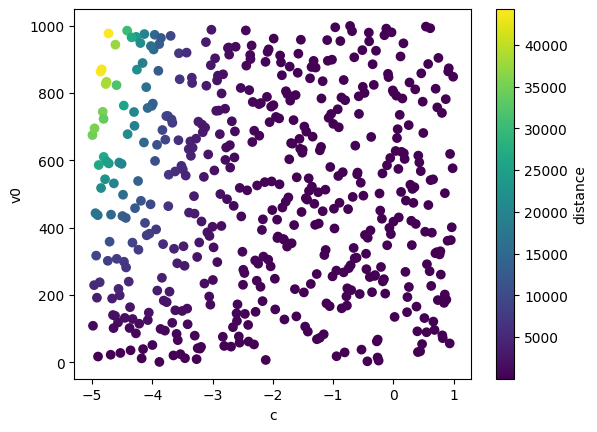
We can also visualize the simulation data before training emulators where the output of the simulator is depicted as the colour of each scatter point.
import matplotlib.pyplot as plt

plt.scatter(x[:, 0], x[:, 1], c=y[:, 0], cmap='viridis')
plt.xlabel(projectile.param_names[0])
plt.ylabel(projectile.param_names[1])
plt.colorbar(label=projectile.output_names[0])
plt.show()
Build and compare Emulators#
With our simulator inputs and outputs, we can run a full machine learning pipeline, including data processing, model fitting, model selection and hyperparameter optimisation in just a few lines of code.
First, let’s import AutoEmulate and check the names of the available Emulator models. The columns indicate whether the emulator has a PyTorch backend, supports multioutput data and provides predictive uncertainty quantification. The list shows only the default set of emulators, but you can also see all available emulators by passing default_only=False to the function.
from autoemulate import AutoEmulate

AutoEmulate.list_emulators()
| Emulator | PyTorch | Multioutput | Uncertainty_Quantification | Automatic_Differentiation | |
|---|---|---|---|---|---|
| 0 | GaussianProcessMatern32 | True | True | True | True |
| 1 | GaussianProcessRBF | True | True | True | True |
| 2 | RadialBasisFunctions | True | True | False | True |
| 3 | PolynomialRegression | True | True | False | True |
| 4 | MLP | True | True | False | True |
| 5 | EnsembleMLP | True | True | True | True |
We’re now ready run AutoEmulate to build and compare emulators.
This will fit (including hyperparameter tuning) emulator models to the simulation input and output to the data, evaluating performance on witheld test data.
# Run AutoEmulate with default settings
ae = AutoEmulate(x, y, show_progress_bar=False)
/home/runner/work/autoemulate/autoemulate/autoemulate/emulators/gaussian_process/exact.py:295: NumericalWarning: cov not p.d. - added 1.0e-05 to the diagonal and symmetrized
  make_positive_definite(
/home/runner/work/autoemulate/autoemulate/autoemulate/emulators/gaussian_process/exact.py:295: NumericalWarning: cov not p.d. - added 1.0e-04 to the diagonal and symmetrized
  make_positive_definite(
For more information about the configuration options available, see the AutoEmulate API docs. Here’s a brief overview of some important options:
Model selection
By default, AutoEmulate will fit all the above listed emulator models, but you can also specify a subset or additional models to use if you already know which kinds of models are most suitable for your data.
Specify models used by AutoEmulate with the models argument, for example:
models = ["GaussianProcessRBF", "GaussianProcessCorrelatedRBF", "RadialBasisFunctions"]
ae = AutoEmulate(x, y, models=models, show_progress_bar=False)
The user can also directly restrict the selection to just probabilistic models by using the only_probabilistic argument without having to list all the models individually:
ae = AutoEmulate(x, y, only_probabilistic=True, show_progress_bar=False)
Metrics
The user can specify what metrics to be used for both the tuning and evaluation. For tuning, only one metric is accepted. This is the metric used to determine which hyperparameter set is the best. For evaluation, multiple metrics can be accepted. These are the metrics reported baack to measure performance on the train and test datasets.
ae = AutoEmulate(x, y, models=models, tuning_metric='r2', evaluation_metrics=['mse', 'r2'], show_progress_bar=False)
Available metrics can be seen by:
from autoemulate.core.metrics import AVAILABLE_METRICS

print(AVAILABLE_METRICS.keys())
Now that we have run AutoEmulate, let’s look at the summary for a comparison of emulator performance (r-squared and RMSE) on both the train and test data.
ae.summarise()
| model_name | x_transforms | y_transforms | params | r2_test | r2_test_std | rmse_test | rmse_test_std | r2_train | r2_train_std | rmse_train | rmse_train_std | |
|---|---|---|---|---|---|---|---|---|---|---|---|---|
| 0 | GaussianProcessMatern32 | [StandardizeTransform()] | [StandardizeTransform()] | {'epochs': 200, 'lr': 0.5, 'likelihood_cls': <... | 0.999987 | 0.000005 | 19.671623 | 3.105990 | 0.999995 | 0.000001 | 16.735819 | 2.190459 |
| 1 | GaussianProcessRBF | [StandardizeTransform()] | [StandardizeTransform()] | {'epochs': 200, 'lr': 0.5, 'likelihood_cls': <... | 0.999978 | 0.000013 | 26.514671 | 2.852429 | 0.999984 | 0.000003 | 30.901749 | 1.982475 |
| 5 | EnsembleMLP | [StandardizeTransform()] | [StandardizeTransform()] | {'n_emulators': 4, 'epochs': 100, 'layer_dims'... | 0.998109 | 0.000842 | 237.493729 | 24.884239 | 0.999126 | 0.000155 | 230.306641 | 14.902583 |
| 2 | RadialBasisFunctions | [StandardizeTransform()] | [StandardizeTransform()] | {'kernel': 'quintic', 'degree': 2, 'smoothing'... | 0.997774 | 0.000857 | 249.983902 | 35.015366 | 0.999052 | 0.000120 | 238.742249 | 16.543310 |
| 4 | MLP | [StandardizeTransform()] | [StandardizeTransform()] | {'epochs': 100, 'layer_dims': [64, 32, 16], 'l... | 0.980958 | 0.007667 | 723.489868 | 93.782501 | 0.990312 | 0.001469 | 760.579712 | 56.407909 |
| 3 | PolynomialRegression | [StandardizeTransform()] | [StandardizeTransform()] | {'lr': 0.1, 'epochs': 500, 'batch_size': 16, '... | 0.704145 | 0.116043 | 2977.205566 | 325.880310 | 0.800312 | 0.020493 | 3450.436279 | 215.870636 |
Choosing an Emulator#
From this list, we can choose an emulator based on the index from the summary dataframe, or quickly get the best performing one using the best_result function, which picks based on the r2_test metric by default.
Choosing a metric for determining the best model
metric_name can be set in the best_result method to choose what metric is used to determine the best model:
ae.best_result(metric_name='rmse')
best = ae.best_result()
print("Model with id: ", best.id, " performed best: ", best.model_name)
Model with id: 0 performed best: GaussianProcessMatern32
best.model.untransformed_model_name
'GaussianProcessMatern32'
Let’s take a look at the configuration of the best model. These are the values of the model’s hyperparameters.
print(best.params)
{'epochs': 200, 'lr': 0.5, 'likelihood_cls': <class 'gpytorch.likelihoods.multitask_gaussian_likelihood.MultitaskGaussianLikelihood'>, 'scheduler_cls': None, 'scheduler_params': {}}
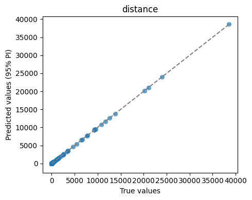
We can quickly visualise the performance of this Emulator with a plot of its predictions against the simulator outputs for the heldout test data. We also save the plot to a file.
ae.plot_preds(best, output_names=projectile.output_names)
/home/runner/work/autoemulate/autoemulate/autoemulate/emulators/gaussian_process/exact.py:295: NumericalWarning: cov not p.d. - added 1.0e-04 to the diagonal and symmetrized
  make_positive_definite(
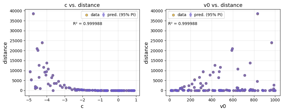
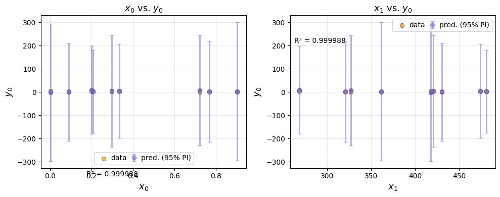
We can also visualise the predictions against each input feature.
ae.plot(best, output_names=projectile.output_names, input_names=projectile.param_names)
/home/runner/work/autoemulate/autoemulate/autoemulate/emulators/gaussian_process/exact.py:295: NumericalWarning: cov not p.d. - added 1.0e-04 to the diagonal and symmetrized
  make_positive_definite(
We can subset the data included in the feature plots by providing input and output ranges.
ae.plot(best, input_ranges={0: (0, 4), 1: (200, 500)}, output_ranges={0: (0, 10)})
/home/runner/work/autoemulate/autoemulate/autoemulate/emulators/gaussian_process/exact.py:295: NumericalWarning: cov not p.d. - added 1.0e-04 to the diagonal and symmetrized
  make_positive_definite(
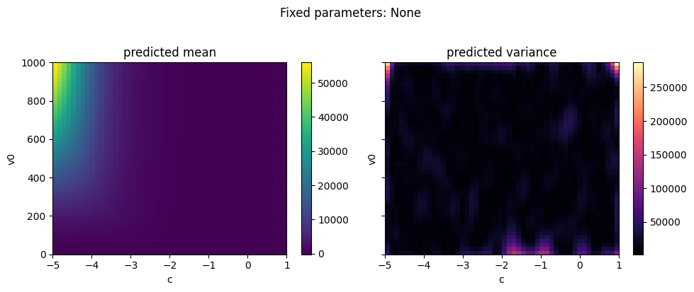
As well as plotting the data, we can directly plot the predicted mean and variance of the emulator for a pair of variables while holding the other variables constant at a given quantile. API to support plotting for a subset of the parameter and output range is also supported.
The emulator predicted mean captures the simulated data plotted at the top of the tutorial well. The predicted variance is low where we have data, and increases away from the data.
ae.plot_surface(best.model, projectile.parameters_range, quantile=0.5)
/home/runner/work/autoemulate/autoemulate/autoemulate/emulators/gaussian_process/exact.py:295: NumericalWarning: cov not p.d. - added 1.0e-04 to the diagonal and symmetrized
  make_positive_definite(
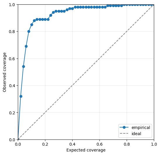
We can also visualise the calibration of the emulator’s predicted uncertainty on the held out test data. The closer the line is to the diagonal, the better calibrated the uncertainty is. Line above the diagonal overestimates the uncertainty while line below the diagonal underestimates it.
ae.plot_calibration(best.model)
Predictions#
We can use the emulator to make predictions using the predict method.
best.model.predict(x[:10])
Independent(Normal(loc: torch.Size([10, 1]), scale: torch.Size([10, 1])), 1)
Saving and loading emulators#
Emulators and their metadata (hyperparameter config and performance metrics) can be saved to disk and loaded again later.
# Make a directory to save Emulator models
import os
path = "my_emulators"
if not os.path.exists(path):
    os.makedirs(path)
Let’s save the best result, the best performing emulator plus metadata, to disk.
# The use_timestamp paramater ensures a new result is saved each time the save method is called
best_result_filepath = ae.save(best, path, use_timestamp=True)
print("Model and metadata saved to: ", best_result_filepath)
Model and metadata saved to: my_emulators/GaussianProcessMatern32_0_20260714_100951
You should now have a two files saved to disk, one with the emulator model and one with the metadata that has the same name and a .csv extension.
You can later pass this filepath to the load_model method to use the model again.
model = AutoEmulate.load_model(best_result_filepath)
model.predict(x[:10])
Independent(Normal(loc: torch.Size([10, 1]), scale: torch.Size([10, 1])), 1)