import matplotlib.pyplot as plt

from autoemulate.emulators import GaussianProcess
from autoemulate.core.compare import AutoEmulate
from autoemulate.simulations.epidemic import Epidemic
from autoemulate.calibration.history_matching import HistoryMatchingWorkflow
from autoemulate.calibration.history_matching_dashboard import HistoryMatchingDashboard

random_seed = 42

History Matching workflow

The HistoryMatching calibration method can be a useful way to iteratively decide which simulations to run to generate data to refine the emulator on. The HistoryMatchingWorkflow implements this iterative sample-predict-refit workflow. Each time it is run:

• parameters are sampled from the not ruled out yet (NROY) space

• an emulator is used in combination with HistoryMatching to score the implausability of the samples

• simulations are run for a subset of the NROY samples

• the emulator is refit given the newly and previously simulated data

In this tutorial, we demonstrate how to use this simulator in the loop workflow.

1. Simulate data and train an emulator

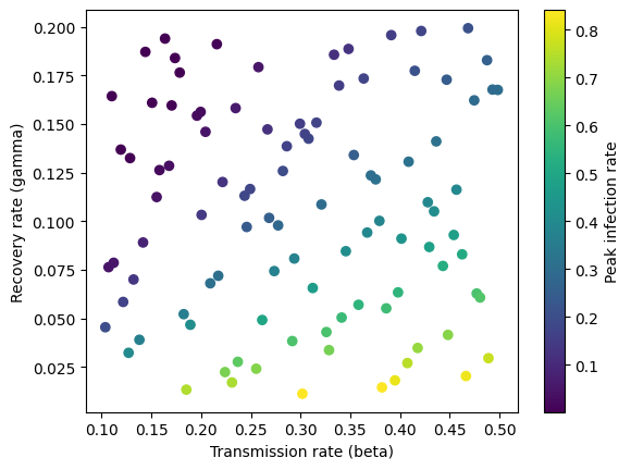
In this example, we’ll use the Epidemic simulator, which returns the peak infection rate given two input parameters, beta(the transimission rate per day) and gamma (the recovery rate per day).

simulator = Epidemic(log_level="error")
x = simulator.sample_inputs(100, random_seed=random_seed)
y, _ = simulator.forward_batch(x)

Below we plot the simulated data. The peak infection rate is higher when the transmission rate increases and the recovery rate decreases and the two parameters are correlated with each other.

transmission_rate = x[:, 0]
recovery_rate = x[:, 1]

plt.scatter(transmission_rate, recovery_rate, c=y, cmap='viridis')
plt.xlabel('Transmission rate (beta)')
plt.ylabel('Recovery rate (gamma)')
plt.colorbar(label="Peak infection rate")
plt.show

<function matplotlib.pyplot.show(close=None, block=None)>

For the purposes of this tutorial, we will restrict the model choice to GaussianProcess with default parameters.

ae = AutoEmulate(
    x,
    y,
    models=[GaussianProcess],
    model_params={},
    log_level="error",
    random_seed=random_seed
)

We can verify that the fitted emulator performs well on both the train and test data.

ae.summarise()

	model_name	x_transforms	y_transforms	params	rmse_test	r2_test	r2_test_std	r2_train	r2_train_std
0	GaussianProcess	[StandardizeTransform()]	[StandardizeTransform()]	{}	0.011999	0.997646	0.001636	0.99987	0.000032

best_result = ae.best_result()

2. Calibrate

To instantiate the HistoryMatchingWorkflow object, we need an observed mean and, optionally, variance for each simulator output.

observations = {"infection_rate": (0.15, 0.05**2)}

In addition to the observations, we pass the fitted emulator and the simulator to the HistoryMatchingWorkflow object at initialisation.

Other options inputs include the history matching parameters (e.g., implausability threshold) and the original training data used to fit the emulator, which can then be used in refitting the emulator in combination with the newly simulated data.

hmw = HistoryMatchingWorkflow(
    simulator=simulator,
    result=best_result,
    observations=observations,
    # optional parameters
    threshold=3.0,
    random_seed=random_seed,
    train_x=x,
    train_y=y
)

The run method implements the sample-predict-refit workflow:

• sample n_test_samples to test from the not ruled out yet (NROY) space

• use emulator to filter out implausible samples and update the NROY space

• run n_simulations predictions for the sampled parameters using the simulator

• refit the emulator using the newly simulated data (unless refit_emulator is set to False)

The HistoryMatchingWorkflow object maintains and updates the internal state each time run() is called, including saving the newly simulated data. This means the full workflow can be run over a number of iterations by calling run repeatedly. At the end of each run the emulator is refit on all data simulated so far (unless refit_on_all_data is set to False).

Alternatively, one can use the run_waves method to run multiple waves of the history matching workflow in one go.

_ = hmw.run_waves(n_waves=1, n_simulations=50, n_test_samples=1000)

3. Visualise results

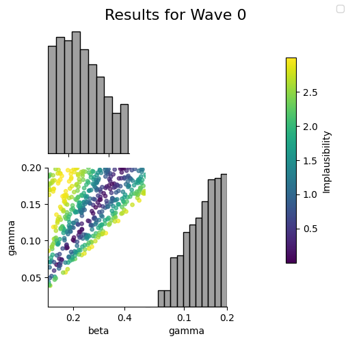
The plot_wave method plots the NROY samples and their implausability scores. There is also an associated plot_run method which takes in as input the outputs of the run method.

hmw.plot_wave(0)

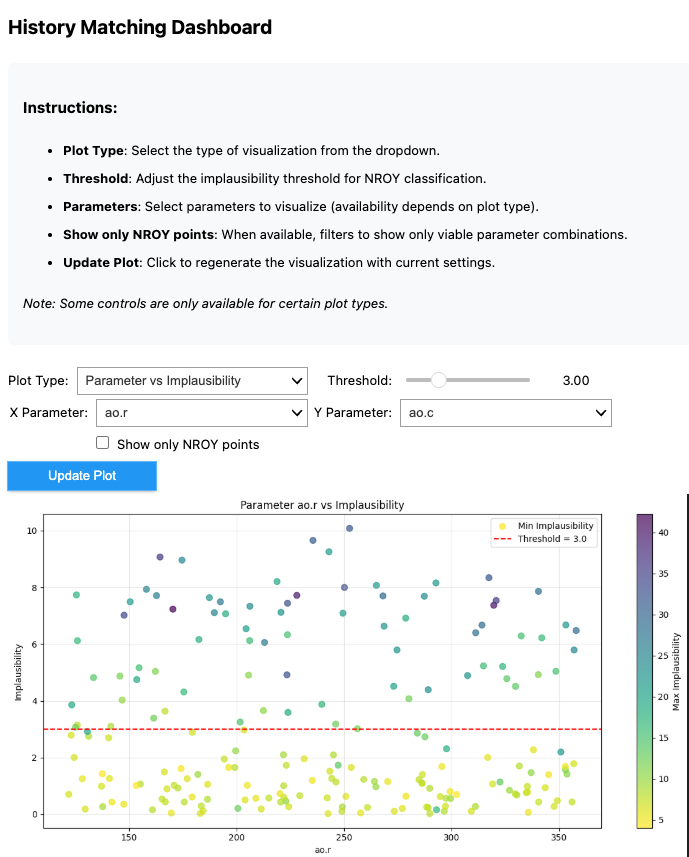
4. Interactive dashboard

HistoryMatchingDashboard implements a number of interactive plots for results exploration. To initialize it just pass in information about the simulation and results for the history matching wave to plot. These are either the outputs returned by the run() or get_wave_results method.

test_parameters, impl_scores = hmw.get_wave_results(0)

dashboard = HistoryMatchingDashboard(
    samples=test_parameters,
    impl_scores=impl_scores,
    param_names=simulator.param_names,  
    output_names=simulator.output_names, 
)

The plots can be viewed using the display() method. Below you can see an example image of what the dashboard looks like.

# dashboard.display()