# probabilistic programming
import pyro 

# MCMC plotting
import arviz as az
import matplotlib.pyplot as plt
from getdist import plots

# autoemulate imports
from autoemulate.calibration.interval_excursion_set import IntervalExcursionSetCalibration
from autoemulate.core.compare import AutoEmulate
from autoemulate.data.utils import set_random_seed
from autoemulate.simulations.projectile import Projectile
from autoemulate.emulators.gaussian_process.exact import GaussianProcessRBF

# random seed for reproducibility
random_seed = 42
set_random_seed(random_seed)
pyro.set_rng_seed(random_seed)

Interval Excursion Set

In this tutorial we will demonstrate how to use AutoEmulate to estimate the interval excursion set of a simulator. The interval excursion set is the set of input parameters for which selected simulator outputs lie within specified intervals. This is a more general problem than estimating level sets, superlevel sets, or sublevel sets, as it allows for the specification of both lower and upper bounds on selected outputs.

We will use the Projectile simulator from the previous tutorials. We will first generate training data and fit a Gaussian process (GP) model to the data. We will then formulate the interval excursion set as a probabilistic model and then use the IntervalExcursionSetCalibration class to estimate the interval excursion set using both gradient-based MCMC (NUTS) and Sequential Monte Carlo (SMC) sampling methods.

Projectile simulation: run simulator and fit emulator

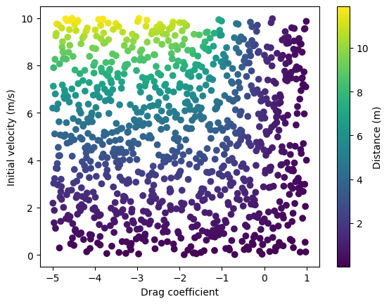
To begin with we create a simulator and generate some training data, before fitting a Gaussian process (GP) emulator to the data using AutoEmulate.

# Create simulator and generate training data
simulator = Projectile(
    parameters_range={"c": (-5.0, 1.0), "v0": (0.0, 10.0)},
    show_progress_bar=False,
)
x = simulator.sample_inputs(1000)
y, _ = simulator.forward_batch(x)

# Visualize training data
c = x[:, 0]
v0 = x[:, 1]
plt.scatter(c, v0, c=y[:, 0], cmap='viridis')
plt.xlabel('Drag coefficient')
plt.ylabel('Initial velocity (m/s)')
plt.colorbar(label="Distance (m)")
plt.show()

# Run AutoEmulate to find the best GP model
ae = AutoEmulate(
    x, 
    y, 
    models=[GaussianProcessRBF],
    model_params={},
    show_progress_bar=False, 
)

# Get best GP model
gp = ae.best_result().model

/home/runner/work/autoemulate/autoemulate/autoemulate/emulators/gaussian_process/exact.py:295: NumericalWarning: cov not p.d. - added 1.0e-05 to the diagonal and symmetrized
  make_positive_definite(
/home/runner/work/autoemulate/autoemulate/autoemulate/emulators/gaussian_process/exact.py:295: NumericalWarning: cov not p.d. - added 1.0e-04 to the diagonal and symmetrized
  make_positive_definite(

Problem set-up: identify an interval excursion set for \(f(\mathbf{x})\)

The aim for the remainder of this notebook is to explore methods that are able to identify samples \(\mathbf{x}\) from the interval excursion set.

Let \(f: \mathbb{R}^n \to \mathbb{R}^m\) be the simulator, and let \(\mathcal{C} \subseteq \{1,\dots,m\}\) index the output components whose intervals are specified. We only need bounds for those components, so \(\mathbf{a}_{\mathcal{C}}, \mathbf{b}_{\mathcal{C}} \in \mathbb{R}^{|\mathcal{C}|}\).

Mathematically this is:

\[ \mathbf{x} \in \mathbb{R}^n, \quad a_k < f_k(\mathbf{x}) < b_k \;\; \forall k \in \mathcal{C} \]

with the interval excursion defined as:

\[ \text{Interval Excursion Set (IES):} \quad \mathrm{IES}_{\mathbf{a}_{\mathcal{C}},\mathbf{b}_{\mathcal{C}},\mathcal{C}} := \{\, \mathbf{x} \in \mathbb{R}^n : a_k < f_k(\mathbf{x}) < b_k \;\; \forall k \in \mathcal{C} \,\} \]

The interval excursion set encompasses, as special cases, several familiar constructions:

• the level set defined by \(f_k(\mathbf{x}) = c\),

• the superlevel set defined by \(f_k(\mathbf{x}) > c\), and

• the sublevel set defined by \(f_k(\mathbf{x}) < c\).

For a single constrained output, if \(y_k \mid \mathbf{x} \sim \mathcal{N}(\mu_k(\mathbf{x}), \sigma_k^2(\mathbf{x}))\), the probability that it lies in the interval \(a_k < y_k < b_k\) is:

\[ p(a_k < y_k < b_k \mid \mathbf{x}) = \Phi\left(\frac{b_k - \mu_k(\mathbf{x})}{\sigma_k(\mathbf{x})}\right) - \Phi\left(\frac{a_k - \mu_k(\mathbf{x})}{\sigma_k(\mathbf{x})}\right) \]

where \(\Phi(\cdot)\) is the cumulative distribution function (CDF) of the standard normal distribution.

For a set of constrained outputs \(\mathcal{C}\), the likelihood used here is the product of these marginal interval probabilities:

\[ p(\mathbf{a}_{\mathcal{C}} < \mathbf{y}_{\mathcal{C}} < \mathbf{b}_{\mathcal{C}} \mid \mathbf{x}) = \prod_{k \in \mathcal{C}} \left[\Phi\left(\frac{b_k - \mu_k(\mathbf{x})}{\sigma_k(\mathbf{x})}\right) - \Phi\left(\frac{a_k - \mu_k(\mathbf{x})}{\sigma_k(\mathbf{x})}\right)\right] \]

This product is taken only over the output dimensions with specified bounds.

In the Bayesian setting, this interval probability is used as a likelihood function. The posterior density for \(\mathbf{x}\) is then proportional to the product of the prior \(p(\mathbf{x})\) and the probability that the constrained model outputs lie within their specified intervals:

\[p(\mathbf{x} \mid \mathbf{a}_{\mathcal{C}} < f_{\mathcal{C}}(\mathbf{x}) < \mathbf{b}_{\mathcal{C}}) \propto p(\mathbf{x}) \prod_{k \in \mathcal{C}} \left[\Phi\left(\frac{b_k - \mu_k(\mathbf{x})}{\sigma_k(\mathbf{x})}\right) - \Phi\left(\frac{a_k - \mu_k(\mathbf{x})}{\sigma_k(\mathbf{x})}\right)\right]\]

where \(\mu_k(\mathbf{x})\) and \(\sigma_k(\mathbf{x})\) are the emulator mean and standard deviation for output component \(k\) at \(\mathbf{x}\).

In this example, Projectile has a single output, distance, so the constrained set \(\mathcal{C}\) contains one component. For a multi-output simulator, the same API supports multiple constrained outputs by passing more entries to output_bounds. For example, if using ProjectileMultioutput, whose outputs are distance and impact_velocity, you could pass {"distance": (6.0, 8.0), "impact_velocity": (2.0, 4.0)}.

lower, upper = 6.0, 8.0
ies = IntervalExcursionSetCalibration(
    gp,
    parameters_range=simulator.parameters_range,
    output_bounds={"distance": (lower, upper)},
    output_names=simulator.output_names,
)

Interval excursion set samples using MCMC

We next run the MCMC sampler. By default, it uses NUTS here, but Metropolis can also produce reasonable samples for low-dimensional parameter spaces, as is the case in this projectile simulator model.

mcmc = ies.run_mcmc(
    num_samples=500,
    warmup_steps=200,
    num_chains=2,
    sampler="nuts",
    # sampler="metropolis",
    model_kwargs={"uniform_prior": True}
)
az_mcmc = ies.to_arviz(mcmc)

/home/runner/work/autoemulate/autoemulate/autoemulate/emulators/gaussian_process/exact.py:295: NumericalWarning: cov not p.d. - added 1.0e-05 to the diagonal and symmetrized
  make_positive_definite(

/home/runner/work/autoemulate/autoemulate/autoemulate/emulators/gaussian_process/exact.py:295: NumericalWarning: cov not p.d. - added 1.0e-05 to the diagonal and symmetrized
  make_positive_definite(

/home/runner/work/autoemulate/autoemulate/autoemulate/emulators/gaussian_process/exact.py:295: NumericalWarning: cov not p.d. - added 1.0e-04 to the diagonal and symmetrized
  make_positive_definite(

/home/runner/work/autoemulate/autoemulate/autoemulate/emulators/gaussian_process/exact.py:295: NumericalWarning: cov not p.d. - added 1.0e-04 to the diagonal and symmetrized
  make_positive_definite(

/home/runner/work/autoemulate/autoemulate/.venv/lib/python3.12/site-packages/arviz/data/io_pyro.py:158: UserWarning: Could not get vectorized trace, log_likelihood group will be omitted. Check your model vectorization or set log_likelihood=False
  warnings.warn(

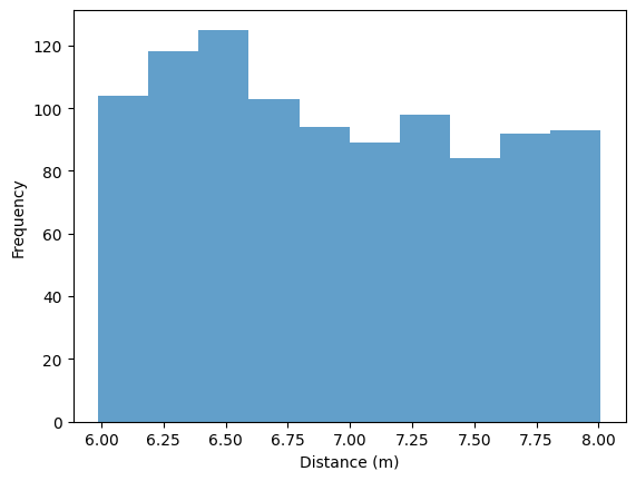
Draw posterior predictive samples.

y_pred = ies.posterior_predictive(mcmc)
plt.hist(y_pred["distance"], density=False, alpha=0.7)
plt.xlabel("Distance (m)")
plt.ylabel("Frequency")
plt.show()

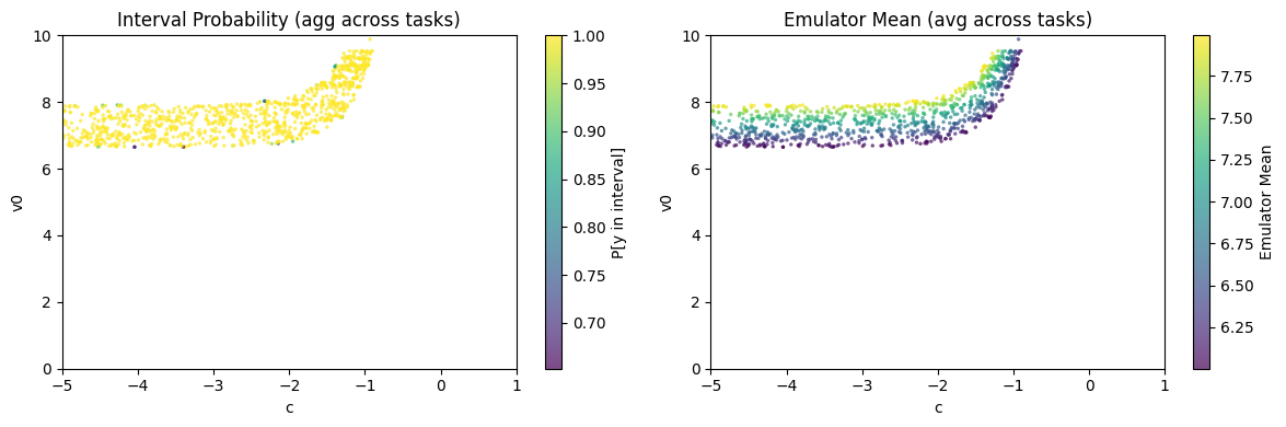
Plot likelihood and mean of MCMC samples.

ies.plot_samples(az_mcmc)

/home/runner/work/autoemulate/autoemulate/autoemulate/emulators/gaussian_process/exact.py:295: NumericalWarning: cov not p.d. - added 1.0e-05 to the diagonal and symmetrized
  make_positive_definite(

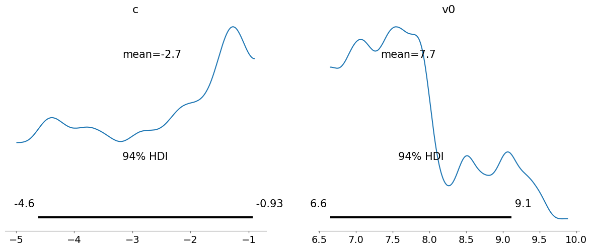
Convert to arviz InferenceData object for further analysis, such as plot_posterior().

az_data = ies.to_arviz(mcmc)
_ = az.plot_posterior(az_data)

/home/runner/work/autoemulate/autoemulate/.venv/lib/python3.12/site-packages/arviz/data/io_pyro.py:158: UserWarning: Could not get vectorized trace, log_likelihood group will be omitted. Check your model vectorization or set log_likelihood=False
  warnings.warn(

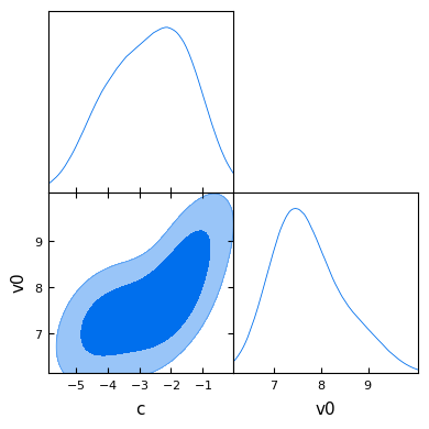
GetDist can also be used to create a plot of posterior sample densities.

def get_dist_and_plot(ies, data):
    """Convert and plot GetDist MCSamples from MCMC samples."""
    emu_data = ies.to_getdist(data, label="Emulator")
    emu_data.smooth_scale_1D = 0.8
    g = plots.get_subplot_plotter()
    g.triangle_plot([emu_data], filled=True)
    plt.show()

get_dist_and_plot(ies, mcmc)

Removed no burn in

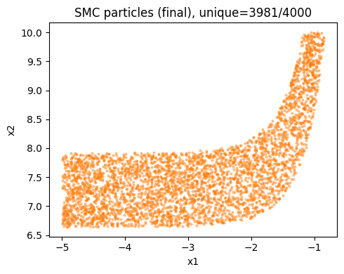
Interval excursion set samples using SMC with adaptive tempering

The Sequential Monte Carlo (SMC) implementation provides an alternative to MCMC approaches.

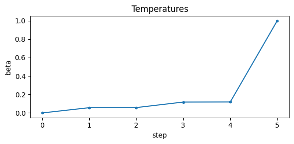
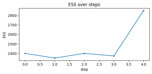
It works by tempering the interval excursion set likelihood from 0 to 1 (i.e. sampling from the prior to the posterior), adaptively controlling steps to hit a target Effective Sample Size (ESS). We resample when ESS falls below the threshold. This converges to the exact target at temperature 1 without gradients.

# Run SMC and plot diagnostics
az_data_smc = ies.run_smc(
    n_particles=4000,
    ess_target_frac=0.6,
    move_steps=2,
    rw_step=0.25,
    seed=random_seed,
    uniform_prior=True,
    plot_diagnostics=True,
    return_az_data=True
)

/home/runner/work/autoemulate/autoemulate/autoemulate/emulators/gaussian_process/exact.py:295: NumericalWarning: cov not p.d. - added 1.0e-04 to the diagonal and symmetrized
  make_positive_definite(

/home/runner/work/autoemulate/autoemulate/autoemulate/emulators/gaussian_process/exact.py:295: NumericalWarning: cov not p.d. - added 1.0e-05 to the diagonal and symmetrized
  make_positive_definite(

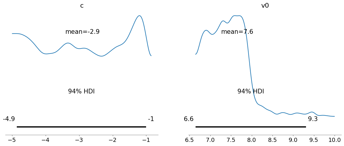
plot_posterior() for SMC samples.

_ = az.plot_posterior(az_data_smc)

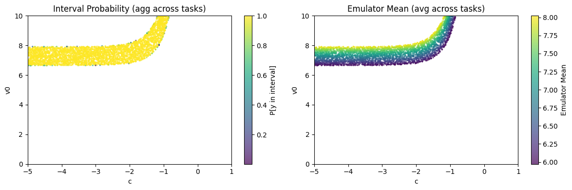
Plot the likelihood and values of SMC samples.

assert isinstance(az_data_smc, az.InferenceData)
ies.plot_samples(az_data_smc)

/home/runner/work/autoemulate/autoemulate/autoemulate/emulators/gaussian_process/exact.py:295: NumericalWarning: cov not p.d. - added 1.0e-04 to the diagonal and symmetrized
  make_positive_definite(

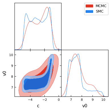
And finally a GetDist plot comparing the MCMC and SMC posterior sample densities. Some differences are expected due to the different sampling approaches, but overall the posterior sample densities are similar.

assert isinstance(az_data_smc, az.InferenceData)
g = plots.get_subplot_plotter()
_ = g.triangle_plot( 
    [ies.to_getdist(az_mcmc, "MCMC"), ies.to_getdist(az_data_smc, "SMC")],
    filled=True,
)

Removed no burn in
Removed no burn in