import torch

# probabilistic programming
import pyro 

# MCMC plotting
import arviz as az
import matplotlib.pyplot as plt
from getdist.arviz_wrapper import arviz_to_mcsamples
from getdist import plots

# autoemulate imports
from autoemulate.simulations.epidemic import Epidemic
from autoemulate.core.compare import AutoEmulate
from autoemulate.calibration.bayes import BayesianCalibration
from autoemulate.emulators import GaussianProcess

# suppress warnings in notebook for readability
import os
import warnings

# ignore warnings
warnings.filterwarnings("ignore")
os.environ["PYTHONWARNINGS"] = "ignore"

# random seed for reproducibility
random_seed = 42

from autoemulate.data.utils import set_random_seed
set_random_seed(random_seed)
pyro.set_rng_seed(random_seed)

Bayesian calibration

Bayesian calibration is a method for estimating which input parameters were most likely to produce observed data. An advantage over other calibration methods is that it returns a probability distribution over the input parameters rather than just point estimates.

Performing Bayesian calibration requires:

• a simulator or an emulator trained to approximate the simulator

• observations associated with the simulator/emulator output

1. Simulate data

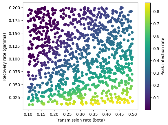
In this example, we’ll use the Epidemic simulator, which returns the peak infection rate given two input parameters, beta(the transimission rate per day) and gamma (the recovery rate per day).

simulator = Epidemic(log_level="error")
x = simulator.sample_inputs(1000)
y, _ = simulator.forward_batch(x)

Below we plot the simulated data. The peak infection rate is higher when the transmission rate increases and the recovery rate decreases and the two parameters are correlated with each other.

transmission_rate = x[:, 0]
recovery_rate = x[:, 1]

plt.scatter(transmission_rate, recovery_rate, c=y, cmap='viridis')
plt.xlabel('Transmission rate (beta)')
plt.ylabel('Recovery rate (gamma)')
plt.colorbar(label="Peak infection rate")
plt.show

<function matplotlib.pyplot.show(close=None, block=None)>

Calibration requires at least one or multiple observations. These can come from running experiments or from the literature.

Below we pick the initial parameter values and simulate the output. We then add noise to generate 100 “observations”.

true_beta = 0.3
true_gamma = 0.15 

# simulator expects inputs of shape [1, number of inputs]
params = torch.tensor([true_beta, true_gamma]).view(1, -1)
true_infection_rate = simulator.forward(params)

n_obs = 100
stdev = 0.05
noise = torch.normal(mean=0, std=stdev, size=(n_obs,))
observed_infection_rates = true_infection_rate[0] + noise

observations = {"infection_rate": observed_infection_rates}

We can now use these observations to infer which input parameters were most likely to have produced them.

2. Calibrate with simulator

In this example, we have a fast simulator with only two input parameters, so we can use the simulator for calibration. The below code shows how to do this directly with Pyro. We can then compare this approach with using an emulator for calibration.

import pyro.distributions as dist
from pyro.infer import MCMC
from pyro.infer.mcmc import RandomWalkKernel

# define the probabilistic model
def model():
    # uniform priors on parameters range
    beta = pyro.sample("beta", dist.Uniform(0.1, 0.5))
    gamma = pyro.sample("gamma", dist.Uniform(0.01, 0.2))
    
    mean = simulator.forward(torch.tensor([[beta, gamma]]))

    with pyro.plate(f"data", n_obs):
        pyro.sample(
            "infection_rate",
            dist.Normal(mean, stdev),
            obs=observations["infection_rate"],
        )

# run Bayesian inference with MCMC


kernel = RandomWalkKernel(model, init_step_size=2.5)
mcmc_sim = MCMC(
    kernel,
    warmup_steps=500,
    num_samples=5000,
    num_chains=1
)
mcmc_sim.run()

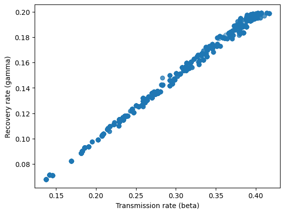
Below we plot the posterior samples of the input parameters.

sim_samples = mcmc_sim.get_samples()
    
plt.scatter(sim_samples['beta'], sim_samples['gamma'], alpha=0.5)
plt.xlabel('Transmission rate (beta)')
plt.ylabel('Recovery rate (gamma)')
plt.show()

3. Calibrate with emulator

For more complex simulators, it is recommended to first train an emulator to approximate the simulator and then use the emulator for calibration. This is because calibration typically requires thousands of evaluations of the simulator, which can be computationally expensive.

AutoEmulate provides the BayesCalibrator class to perform Bayesian calibration with an emulator.

First we need to train an emulator. For the purposes of this tutorial, we will restrict the emulator choice to GaussianProcess with default hyperparameters.

ae = AutoEmulate(
    x, 
    y, 
    models=[GaussianProcess], 
    # use default parameters
    model_params={},
    log_level="error", 
)

We can verify that the fitted emulator performs well on both the train and test data.

ae.summarise()

	model_name	x_transforms	y_transforms	params	rmse_test	r2_test	r2_test_std	r2_train	r2_train_std
0	GaussianProcess	[StandardizeTransform()]	[StandardizeTransform()]	{}	0.001094	0.999977	0.000005	0.999974	0.000003

gp = ae.best_result().model

The BayesianCalibration object takes as input the trained emulator, the simulator parameter ranges and the “observed” data simulated above.

The underlying probabilistic model is the same one used on the simulator example above. It assumes the observations are drawn from a Gaussian distribution with the mean predicted by the emulator. The user also has to specify the observation_noise which is the variance of the Gaussian likelihood.

bc = BayesianCalibration(
    gp, 
    simulator.parameters_range, 
    observations, 
    # specify noise as variance
    observation_noise=stdev**2
)

Run MCMC using the NUTS sampler. The BayesianCalibration class uses Pyro under the hood. Below we use pyro.set_rng_seed to ensure reproducibility.

mcmc_emu = bc.run_mcmc(
    warmup_steps=250, 
    num_samples=1000,
    num_chains=2    
)

The above returns the Pyro MCMC object which has a number of useful methods associated with it. One can access all the posterior samples using mcmc.get_samples() or just the summary statistics using mcmc.summary(). This shows that the posterior mean estimates of the input parameters are close to the true values used to generate the observations.

mcmc_emu.summary()

                mean       std    median      5.0%     95.0%     n_eff     r_hat
      beta      0.30      0.07      0.32      0.20      0.41     38.02      1.06
     gamma      0.15      0.04      0.16      0.10      0.20     37.34      1.06

Number of divergences: 9

3. Plotting with Arviz

The BayesianCalibrator.to_arviz method converts the mcmc object so that it is compatible with the Arviz plotting library. Using Arviz makes it very easy to produce all the standard plots of the calibration results as well as MCMC diagnostics.

az_data = bc.to_arviz(mcmc_emu, posterior_predictive=True)

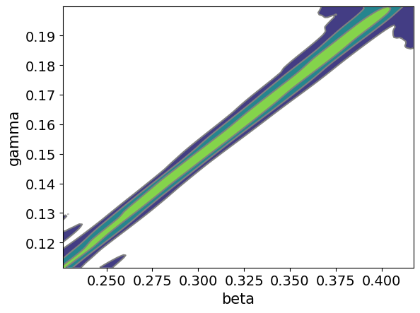
The main plot of interest is the posterior distribution over the parameters given the observations. Below we plot the pairwise joint distribution and can see that the two parameters are correlated as expected. The results look very similar to the results obtained using the simulator directly above.

_ = az.plot_pair(az_data, kind='kde')

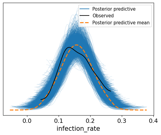
The posterior predictive samples can be plotted alongside the observed data. This shows that the calibration results capture the observed data well.

_ = az.plot_ppc(az_data)

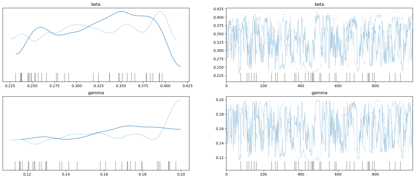
To check the MCMC behaviour, the samples from the posterior distribution can be viewed as a trace (right-hand plots) with 1D KDEs for each chain for each variable (left-hand plots).

_ = az.plot_trace(az_data, figsize=(20, 8))

4. Plotting with GetDist

The BayesianCalibration.to_getdist static method converts an mcmc object so that it is compatible with the getdist plotting library. Alternatively, one can use the arviz_to_mcsamples function from GetDist to convert the Arviz data object to a GetDist MCSamples object.

# convert simulator calibration samples
sim_data = BayesianCalibration.to_getdist(mcmc_sim, label="Simulator")

# convert emulator calibration samples
emu_data = arviz_to_mcsamples(az_data, dataset_label="Emulator")

Removed no burn in
Removed no burn in

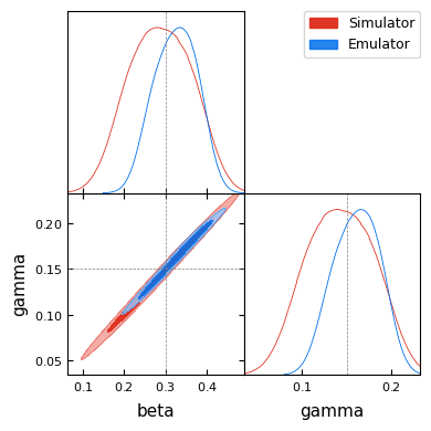
Below we compare the posterior distributions obtained using the simulator and the emulator. Both distributions capture the true parameter values (indicated by the dashed lines).

sim_data.smooth_scale_1D = 0.8
emu_data.smooth_scale_1D = 0.8

g = plots.get_subplot_plotter()
g.triangle_plot( 
    [sim_data, emu_data], 
    filled=True,
    markers={"beta": true_beta, "gamma": true_gamma},
)
plt.show()

# g.fig.savefig("bayes_calibration_getdist.png")