import torch

import matplotlib.pyplot as plt

from autoemulate.emulators import GaussianProcessRBF
from autoemulate.core.compare import AutoEmulate
from autoemulate.simulations.projectile import Projectile
from autoemulate.calibration.history_matching import HistoryMatching
In this tutorial we demonstrate the use of History Matching to determine which points in the input space are plausible given a set of observations.
Performing History Matching requires:
a fit emulator that predicts uncertainty (e.g., Gaussian Process) and
an observation associated with the simulator output.
The emulator is used to efficiently estimate the simulator output, accounting for all uncertainties. The emulated output is then compared with the observation and parameter inputs that are unlikely to produce the observation can then be “ruled out” as implausible, reducing the input space.
History Matching#
1. Simulate data and train an emulator#
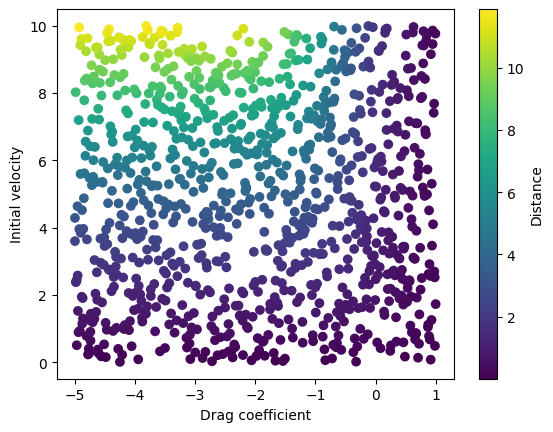
In this example we use the Projectile simulator. It returns distance travelled by a projectile given a drag coefficient c and initial velocity v0.
simulator = Projectile(show_progress_bar=False, parameters_range={'c': (-5.0, 1.0), 'v0': (0.0, 10)})
x = simulator.sample_inputs(1000)
y, _ = simulator.forward_batch(x)
plt.scatter(x[:, 0], x[:, 1], c=y, cmap='viridis')
plt.xlabel('Drag coefficient')
plt.ylabel('Initial velocity')
plt.colorbar(label="Distance")
plt.show
<function matplotlib.pyplot.show(close=None, block=None)>
Since we need an uncertainty aware emulator, we restrict AutoEmulate to only train a Gaussian Process. For the purposes of this tutorial, we use default parameters.
ae = AutoEmulate(x, y, models=[GaussianProcessRBF], model_params={}, show_progress_bar=False)
/home/runner/work/autoemulate/autoemulate/autoemulate/emulators/gaussian_process/exact.py:295: NumericalWarning: cov not p.d. - added 1.0e-05 to the diagonal and symmetrized
  make_positive_definite(
We can verify that the fitted emulator performs well on both the train and test data.
ae.summarise()
| model_name | x_transforms | y_transforms | params | r2_test | r2_test_std | rmse_test | rmse_test_std | r2_train | r2_train_std | rmse_train | rmse_train_std | |
|---|---|---|---|---|---|---|---|---|---|---|---|---|
| 0 | GaussianProcessRBF | [StandardizeTransform()] | [StandardizeTransform()] | {'likelihood_cls': <class 'gpytorch.likelihood... | 0.999991 | 0.000001 | 0.009768 | 0.000477 | 0.999991 | 6.400302e-07 | 0.009305 | 0.000259 |
model = ae.best_result().model
2. Calibrate#
To instantiate the HistoryMatching object, we need an observed mean and, optionally, variance for each simulator output.
true_drag = -2.0
true_velocity = 7.0
distance = simulator.forward(torch.tensor([[true_drag, true_velocity]]))
stdev = distance.item() * 0.05
observation = {"distance": (distance.item(), stdev**2)}
distance
tensor([[6.2728]], dtype=torch.float64)
#  observed data: (mean, variance)
hm = HistoryMatching(observations=observation)
We also need predictions for a set of query points using the trained emulator. These must have uncertainty estimates.
x_new = simulator.sample_inputs(1000)
mean, variance = model.predict_mean_and_variance(x_new)
/home/runner/work/autoemulate/autoemulate/autoemulate/emulators/gaussian_process/exact.py:295: NumericalWarning: cov not p.d. - added 1.0e-05 to the diagonal and symmetrized
  make_positive_definite(
Primary use of the HistoryMatching class is the calculate_implausibility method, which returns the implausibility metric (a number of standard deviations between the emulator mean and the observation) for the queried points.
implausability = hm.calculate_implausibility(mean, variance)

# first 10 implausability scores
implausability[:10]
tensor([[ 7.8094],
        [ 7.6029],
        [14.4983],
        [18.7434],
        [12.9821],
        [ 7.2183],
        [16.8816],
        [12.0642],
        [ 3.6115],
        [10.3916]])
The get_nroy method can be used to filter the queried points given the implausability scores and only retain those that have not been ruled out yet (NROY).
nroy_params = hm.get_nroy(implausability, x_new)
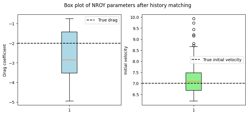
Below we plot the NROY parameters against the true parameters used to generate the observed data. History matching has successfully ruled out a portion of the input space.
fig, ax = plt.subplots(1, 2, figsize=(10, 4))

ax[0].boxplot(nroy_params[:, 0], vert=True, patch_artist=True, boxprops=dict(facecolor='lightblue'))
ax[0].axhline(true_drag, color="k", linestyle="--", label="True drag")
ax[0].set_ylabel("Drag coefficient")
ax[0].legend()

ax[1].boxplot(nroy_params[:, 1], vert=True, patch_artist=True, boxprops=dict(facecolor='lightgreen'))
ax[1].axhline(true_velocity, color="k", linestyle="--", label="True initial velocity")
ax[1].legend()
ax[1].set_ylabel("Initial velocity")

plt.suptitle("Box plot of NROY parameters after history matching")
plt.show()