Reduced-dimension Emulator

Dimensionality reduction overview

Sometimes an emulator performs better when the input and/or the output dimensionality is reduced. In this example, we show how one can try different dimensionality reduction methods in combination with the emulators tested by AutoEmulate.

Reaction-Diffusion example

We train an emulator to generate solutions to a 2D parameterized reaction-diffusion problem governed by the following partial differential equations:

\[ \dot{u} = (1 - (u^2 + v^2)) u + \beta (u^2 + v^2) v + d (u_{xx} + u_{yy}), \]

\[ \dot{v} = -\beta (u^2 + v^2) u + (1 - (u^2 + v^2)) v + d (v_{xx} + v_{yy}), \]

where:

• \( u \) and \( v \) are the concentrations of two species,

• \( \beta \) and \( d \) control the reaction and diffusion terms.

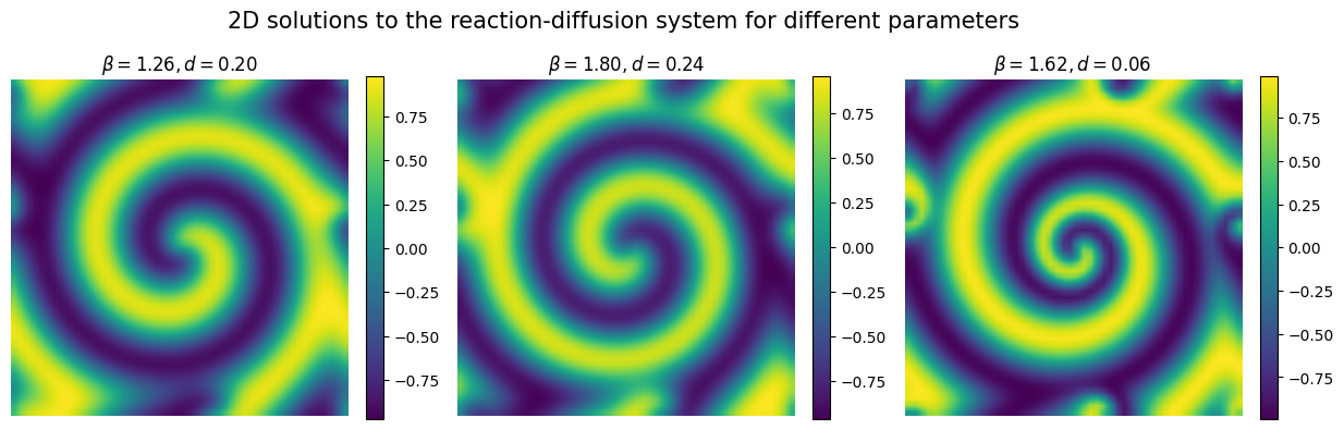
This system exhibits complex spatio-temporal dynamics such as spiral waves.

import numpy as np
import pandas as pd
import matplotlib.pyplot as plt 
import os
import warnings
warnings.filterwarnings("ignore")

from autoemulate.simulations.reaction_diffusion import ReactionDiffusion
from autoemulate.datasets import fetch_data

save = False
train = False

1: Data generation

Data are computed using a numerical simulator using Fourier spectral method. The simulator takes two inputs: the reaction parameter \(\beta\) and the diffusion parameter \(d\).

We sample 50 sets of inputs X using Latin Hypercube sampling and run the simulator for those inputs to get the solutions Y. Below you can either run the simulator or load data that has already been simulated.

n_samples = 50
n = 50
sim = ReactionDiffusion(n=n, T=10)
X = sim.sample_inputs(n_samples)

if train:
    data_folder =  "../data/reactiondiffusion1/processed" 
    if not os.path.exists(data_folder):
        os.makedirs(data_folder)  
    X_file = os.path.join(data_folder, "parameters.csv")
    Y_file = os.path.join(data_folder, "outputs.csv")


    # Run the simulator to generate data 
    # Simulator returns flattened species U and V
    UV = sim.forward_batch(X)

    # Let's consider as output the concentration of species U
    m = int(UV.shape[1] / 2)
    Y = UV[:, :m]

    if save:
        # Save the data
        pd.DataFrame(X).to_csv(X_file, index=False)
        pd.DataFrame(Y).to_csv(Y_file, index=False)
else:
    # Load the data
    X, Y = fetch_data('reactiondiffusion1')

print(f"shapes: input X: {X.shape}, output Y: {Y.shape}\n")

shapes: input X: torch.Size([50, 2]), output Y: torch.Size([50, 2500])

X and Y are matrices where each row represents one run of the simulation. In the input matrix X the two columns indicate the input parameters (reaction \(\beta\) and diffusion \(d\) parameters, respetively). In the output matrix Y each column indicates a spatial location where the solution (i.e. the concentration of \(u\) at final time \(T=10\)) is computed.
We consider a 2D spatial grid of \(50\times 50\) points, therefore each row of Y corresponds to a 2500-dimensional vector!

Let’s now plot the simulated data to see what the reaction-diffusion pattern looks like.

plt.figure(figsize=(15,4.5))
for param in range(3):
  plt.subplot(1,3,1+param)
  plt.imshow(Y[param].reshape(n,n), interpolation='bilinear')
  plt.axis('off')
  plt.xlabel('x', fontsize=12)
  plt.ylabel('y')
  plt.title(r'$\beta = {:.2f}, d = {:.2f}$'.format(X[param][0], X[param][1]), fontsize=12)
  plt.colorbar(fraction=0.046)
plt.suptitle('2D solutions to the reaction-diffusion system for different parameters', fontsize=15)
plt.show()

2: Fit an emulator on a subset of the data

Below we set up a TransformedEmulator object, which takes in an emulator model as well as a sequence on x_transforms and y_transforms. In this example we apply PCA to the simulation output and train a Gaussian Process emulator on this reduced problem space. This is often more efficient for high dimensional problems.

Note that different combinations of x_transforms and y_transforms can be passed directly to the AutoEmulate object before compare() is run, which will test all the different transform combinations with all the emulators. In addition to dimensionality reduction with PCA, AutoEmulate also has an option to use Variational Autoencoder.

from autoemulate.emulators.gaussian_process.exact import GaussianProcess
from autoemulate.emulators.gaussian_process.kernel import rbf_plus_constant
from autoemulate.emulators.gaussian_process.mean import constant_mean
from autoemulate.emulators.transformed.base import TransformedEmulator
from autoemulate.transforms import *
import torch 

# Convert to tensors
x, y = torch.Tensor(X).float(), torch.Tensor(Y).float()

# Create a TransformedEmulator
em = TransformedEmulator(
    x,
    y,
    model= GaussianProcess,
    x_transforms=[StandardizeTransform()],
    y_transforms=[
        StandardizeTransform(),
        PCATransform(n_components=16),
        StandardizeTransform()
    ],
    epochs=50,
    lr=0.2,
    mean_module_fn=constant_mean,
    covar_module_fn=rbf_plus_constant,
    posterior_predictive=True
)

test_idx = [np.array([13, 39, 30, 45, 17, 48, 26, 25, 32, 19])]
train_idx = np.setdiff1d(np.arange(len(x)), test_idx)

# Fit on all data
em.fit(x[train_idx], y[train_idx])

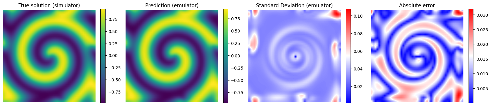
3: Test predictions

# Get predictions for the full dataset
y_true = y[test_idx].numpy()
y_pred_dis = em.predict(x[test_idx])
y_pred = y_pred_dis.mean.numpy()
y_std_pred = y_pred_dis.stddev.numpy()

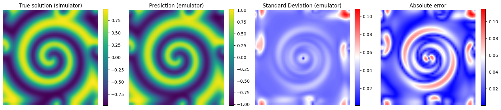
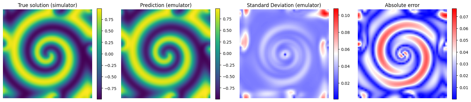
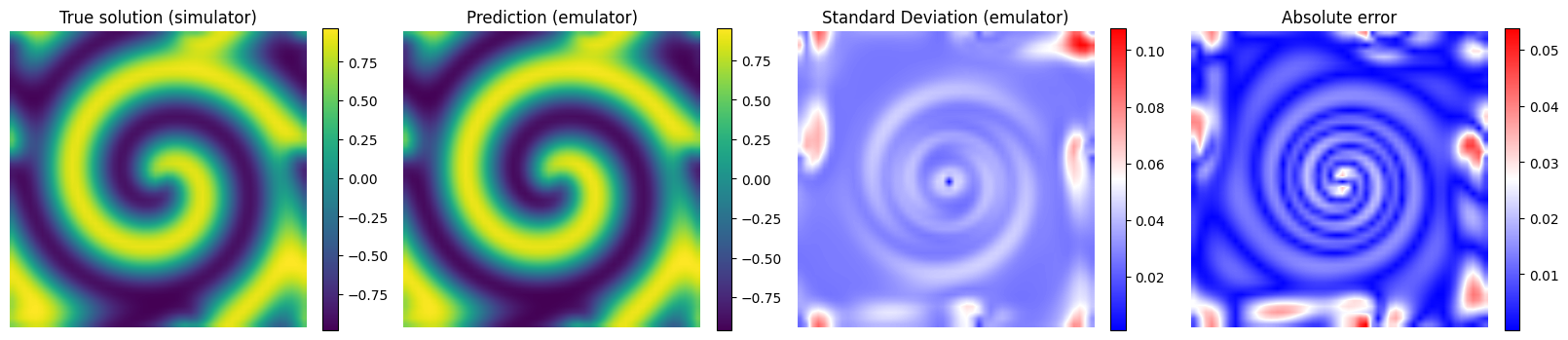
# Plot the results for some unseen (test) parameter instances
params_test = [0,1,2,3]

for param_test in params_test:
  plt.figure(figsize=(20,4.5))
  plt.subplot(1,4,1)
  plt.imshow(y_true[param_test].reshape(n,n), interpolation='bilinear')
  plt.axis('off')
  plt.xlabel('x', fontsize=12)
  plt.ylabel('y')
  plt.title('True solution (simulator)', fontsize=12)
  plt.colorbar(fraction=0.046)

  plt.subplot(1,4,2)
  plt.imshow(y_pred[param_test].reshape(n,n), interpolation='bilinear')
  plt.axis('off')
  plt.xlabel('x', fontsize=12)
  plt.ylabel('y')
  plt.title('Prediction (emulator)', fontsize=12)
  plt.colorbar(fraction=0.046)

  plt.subplot(1,4,3)
  plt.imshow(y_std_pred[param_test].reshape(n,n), cmap = 'bwr', interpolation='bilinear', vmax = np.max(y_std_pred[params_test]))
  plt.axis('off')
  plt.xlabel('x', fontsize=12)
  plt.ylabel('y')
  plt.title('Standard Deviation (emulator)', fontsize=12)
  plt.colorbar(fraction=0.046)

  plt.subplot(1,4,4)
  plt.imshow(np.abs(y_pred[param_test] - y_true[param_test]).reshape(n,n), cmap = 'bwr', interpolation='bilinear')
  plt.axis('off')
  plt.xlabel('x', fontsize=12)
  plt.ylabel('y')
  plt.title('Absolute error', fontsize=12)
  plt.colorbar(fraction=0.046)

  # plt.suptitle(r'Results for test parameters: $\beta = {:.2f}, d = {:.2f}$'.format(X[em.test_idxs][param_test][0], X[em.test_idxs][param_test][1]), fontsize=12)
  plt.show()