Statistical Fairness

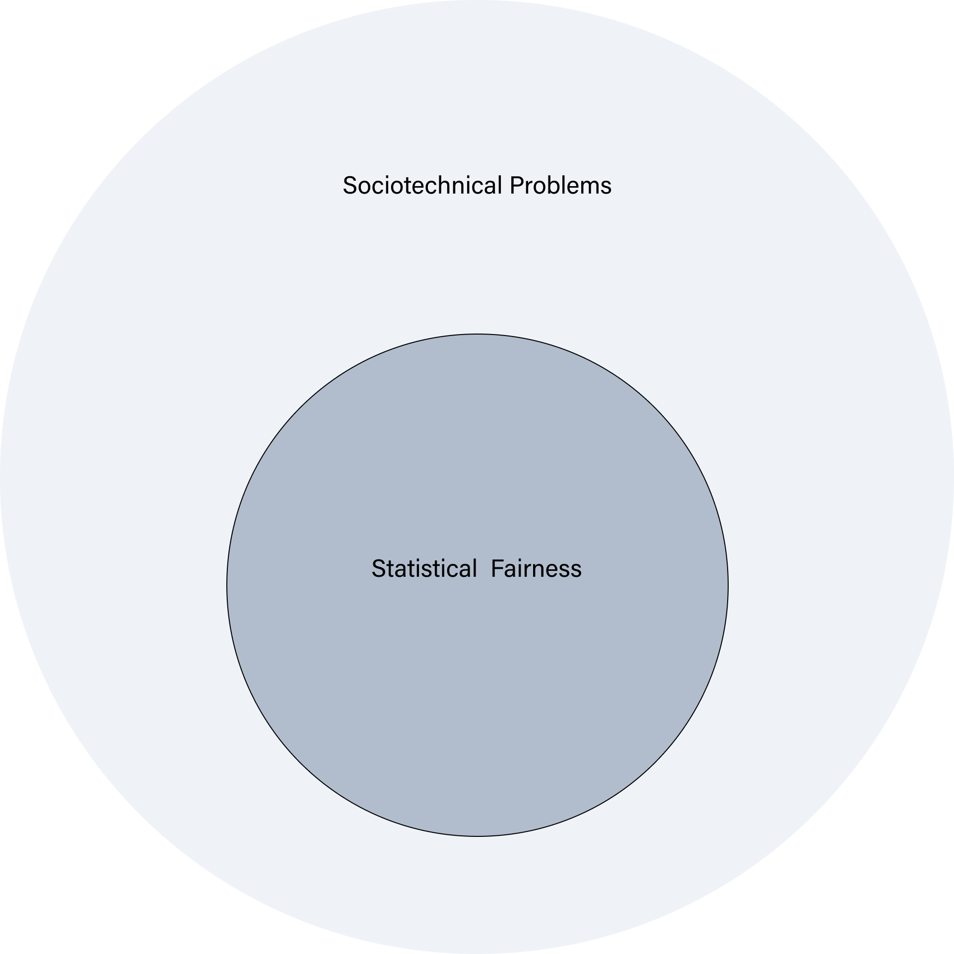
The Computational Allure of Statistical Fairness

Humans have tried to quantify fairness for centuries. The Law of Hammurabi, for example, states that if a man "destroy's the eye of a man's slave or beaks a bone of a man's slave, he shall pay one-half his price".¹ We rightfully recoil at the idea of such a law being espoused and adhered to in modern society. However, the idea that we can quantify fairness is still very much alive, and still not without its problems.

Photograph of the basalt stele with the Law of Hammurabi inscribed (By Mbzt - Own work, CC BY 3.0, https://commons.wikimedia.org/w/index.php?curid=16931676).

Fairness in ML and AI has seen enormous interest over the last decade, as many researchers and developers try to bring conceptual and pragmatic order to a vast and complex landscape of statistical methods and measures. This is understandable. Statistical measures are, typically, well-defined and can bring formal precision or a quantitative dimension to the discussion of fairness.

Attempting to translate fairness into a statistical problem, therefore, has a certain allure because it suggests that if we can get the right measure or formula we can "solve" the problem of fairness in an objective manner. However, the allure of this statistical or computational approach needs to be properly seen for what it is—an important tool, but one that has many limitations and needs to be used responsibly.² This section is about understanding both the strengths and limitations of statistical fairness.

As a simple example of one limitation to get us started, consider the following question:

Question

Is it fair for a company to build an AI system that monitors the performance of employees in a factory and automatically notifies them when they are not meeting their targets? Or, should the company instead invest in better training and support for employees and work with their staff to understand obstacles or barriers?

As you can probably guess, based on the questions posed in the first section of this module, there is no easy answer to this question. In fact, you may have realised that a lot depends on factors that are not appropriately specified in the question (e.g. what happens if the staff continue to miss targets, who is this company, and who are their staff?). However, putting aside these unspecified factors, it should be evident that such a question cannot be reduced solely to a statistical problem.

Problem Formulation

This issue is a key motivator for the dual perspectives required by the Problem Formulation stage in our project lifecycle model.

Here, judging the fairness of the company's actions would require a more holistic approach—one that takes into account the social and cultural context of the company and its staff when defining the problem. Within this more holistic approach, statistical fairness could be an important tool that is used to help inform the discussion, but it will not be the only tool.

Venn diagram showing statistical fairness issues are a subset of wider sociotechnical considerations.

Therefore, in this section we will take a critical look at some proposed statistical concepts and techniques for understanding fairness in ML and AI, paying close attention to how they can contribute to the discussion of fairness, and where they fall short.

Fairness in Classification Tasks

The area of ML and AI that has seen the most attention, with respect to fairness, is the task of classification.

In a classification task, the goal is to predict which class a given input belongs to. This high-level description can be applied to a wide range of tasks, including:

1. Which object is depicted in an image?
2. Is an applicant likely to default on a loan?
3. Is a post on social media an instance of hate speech?
4. Will this patient be readmitted to hospital within 30 days?

Types of Classification Task

These four questions are all instances of classification tasks, but some are instances of binary classification (e.g. yes or no answers) and others are multi-class problems (e.g. which of several classes does an instance or object belong to?).

Do you know which of the four tasks are which?

Answers

1. Multi-class: there are many objects that could be present in an image (e.g. cup, book, cat, dog).
2. Binary: an applicant will either default on a loan or not (within the specified time of the loan agreement)
3. Binary: a post either contains hate speech or it does not
4. Binary/Multi-Class: this question appears to be a binary problem as it is currently framed, but could also be a multi-class problem if there were further buckets (e.g. 5 days, 10 days, 20 days, 30 days).

There are also further complications with some of the other questions. For instance, although (3) is binary, much depends on how 'hate speech' is defined and operationalised. From a statistical perspective, there is a 'yes' or 'no' answer, but this abstraction screens off a lot of societal nuance and disagreement that exists where such clearly defined boundaries are unlikely to exist (e.g. vagueness of social categories).

In this section, we are going to follow this approach and build up our knowledge of statistical fairness by using a simple binary classification task as a running example.

This simplification has a cost and a benefit:

• Cost: we will not be able to capture the full complexity of statistical fairness in ML and AI, such as exploring all relevant metrics, or different types of problems (e.g. multi-class classification, non-classification tasks, etc.)
• Benefit: we will be able to focus more closely on key concepts and ideas and link them to ethical and social issues of fairness.

This trade-off is appropriate for our present purposes, as we are primarily interested in responsible research and innovation, rather than, say, learning how to implement statistical fairness criteria in Python. Therefore, with these caveats in mind, let's dive in.

Classifying Patients: A Running Example

First of all, let's introduce our classification task:

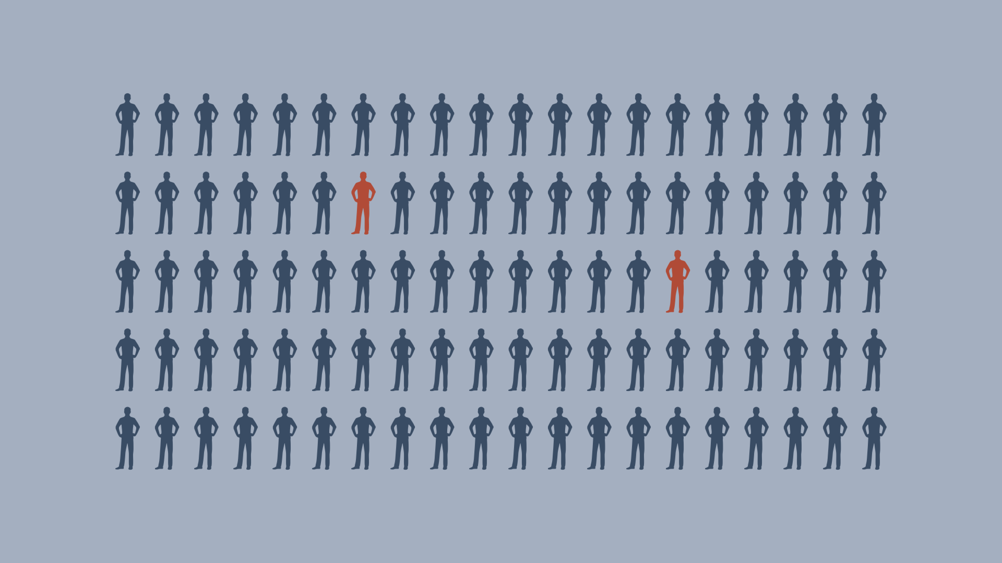
A project team are developing a classification model, using supervised learning. The model will try to predict whether a patient has a disease or not based on a set of features. We're not going to worry about what this disease may be or which features are being used to train the model—our first oversimplification. Instead, let's just assume the training data contains information about 100 patients and 2 of them are known to have the disease.

Graphic showing a population of one hundred people, with two of them sick (depicted in red).

Statistical Fairness Issue #1: Class Imbalance and Accuracy

When designing this model, the project team may decide that evaluating the performance of this model is best achieved by measuring its accuracy.

However, this is where we come to our first problem that statistical fairness has to address: class imbalance.

In our sample of 100 patients, only 2 of them have the disease. These two patients represent our positive class and are a clear minority when compared to the negative class (i.e. those who do not have the disease).

Positive Classes

In ML classification, the term 'positive class' is used to refer to the class that we want to identify or predict.
For example, in a medical diagnosis task, the positive class might represent the presence of a particular disease, while the negative class represents its absence.

This can sometimes cause confusion, as the term 'positive' is often used to refer to something that is good or desirable, but in some tasks the identification of the positive class may be related to an undesirable or negative outcome.

Because of this imbalance between our two classes, if we were to build an (admittedly terrible) model that always predicted that a patient does not have the disease (i.e. classifies all patients as belonging to the negative class), then the model would have an overall accuracy of 98%. From one (very limited) perspective, the model would be performing very well, but we obviously know that this is not the case.

When we have imbalanced classes (i.e. a small number of positive examples), which is quite common in real-world data, such a simplistic notion of accuracy is not going to be sufficient. Fortunately, there is a well-understood approach to dealing with this initial limited notion of accuracy: a confusion matrix that displays additional performance metrics.

Illustration showing that having balanced classes is important for optimal model performance.

A confusion matrix is a table that helps us to visualise the performance of a classification model by showing where it is doing well and what errors it is making. The table below shows a typical confusion matrix, where the columns represent the predicted label (i.e. the model's prediction) and the rows represent the ground truth (i.e. the actual state of the world).

	Predicted Positive	Predictive Negative
Actual Positive	True Positive (TP)	False Negative (FN)
Actual Negative	False Positive (FP)	True Negative (TN)

Table 1: Confusion matrix

Different Terminology

Depending on your background, you may know some of the terms in this section by different names.
For example, 'False Positive' is sometimes referred to as a 'Type I Error', and 'False Negative' is sometimes referred to as a 'Type II Error'.

This will also hold true for terms we define later in the section—an unfortunate, but unavoidable occurrence in such a multi-disciplinary context.

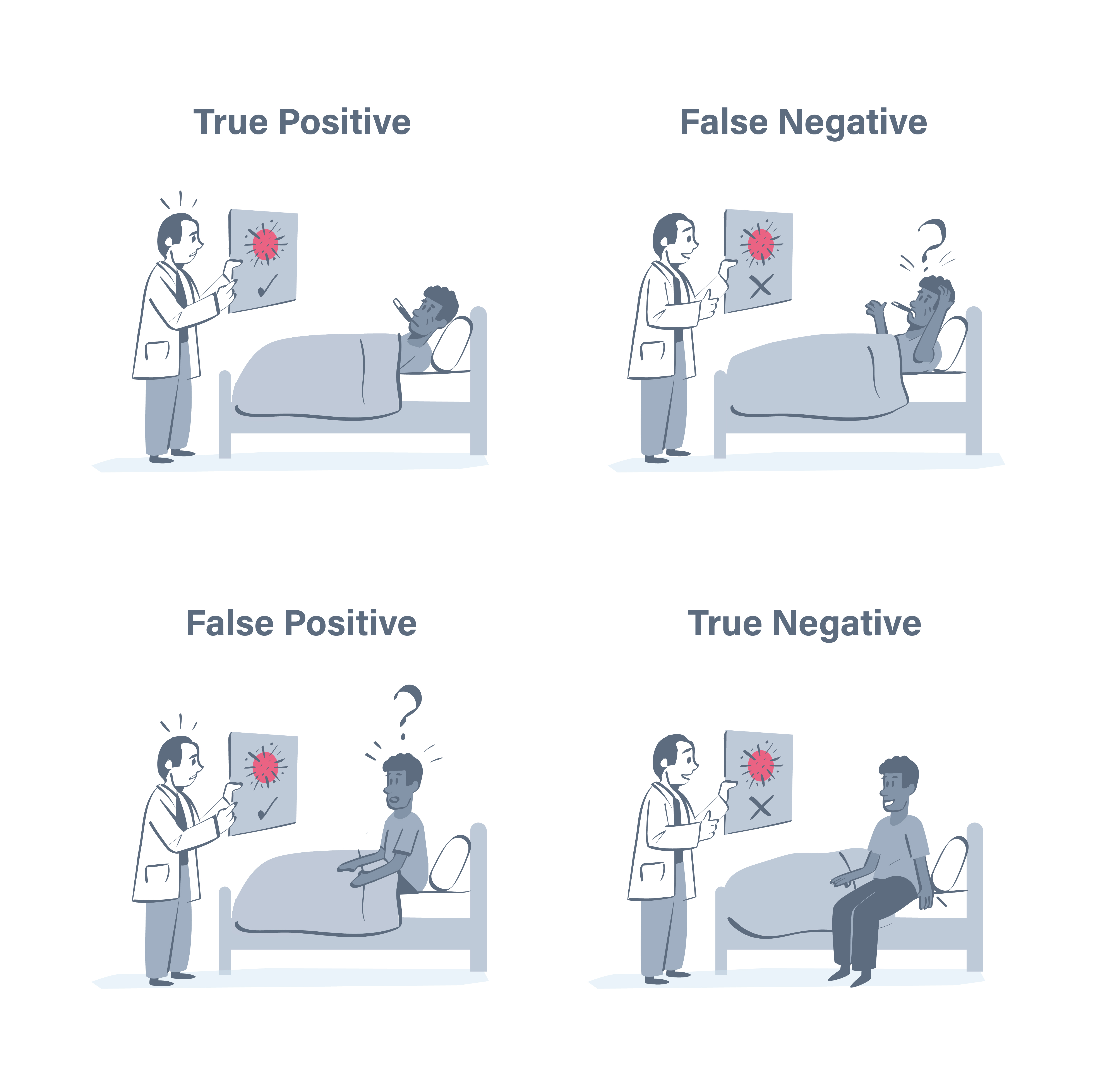
Let's translate this general table into our running example.

Here, the positive class is the presence of the disease, while the negative class is the absence of the disease. Therefore, the four cells would correspond to the following:

• True Positive (TP): The model correctly predicts (T) that the patient has the disease (P).
• False Positive (FP): The model incorrectly predicts (F) that the patient has the disease (P) when they do not.
• False Negative (FN): The model incorrectly predicts (F) that they do not have the disease (N) when they do.
• True Negative (TN): The model correctly predicts (T) that the patient does not have the disease (N).

Illustration of a confusion matrix using the prediction of a disease as an example.

Prediction and Reality

It is common to distinguish between the class predicted by the model and the actual state of affairs by using the following formal convention:

- $Y$: the actual value (e.g. presence of disease)
- $\hat{Y}$: the predicted value (e.g. prediction of disease)

Here, $Y$ and $\hat{Y}$ take the values $1$ or $0$ depending on whether the patient has (or is predicted to have) the disease ($1$) or not ($0$) respectively.
We will return to these variables later.

We can also represent this visually based on how our model performs with respect to the original dataset. Let's return to our original 100 patients, but this time let's make the disease a bit more prevalent, and let's see how well our model does at predicting the disease this time around.

Graphic showing the outcome of a classification task. The model correctly classified 65 out of 70 healthy people as healthy, and 25 out of 35 sick people as sick. However, it incorrectly classified 5 healthy people as sick, and 5 sick people as healthy.

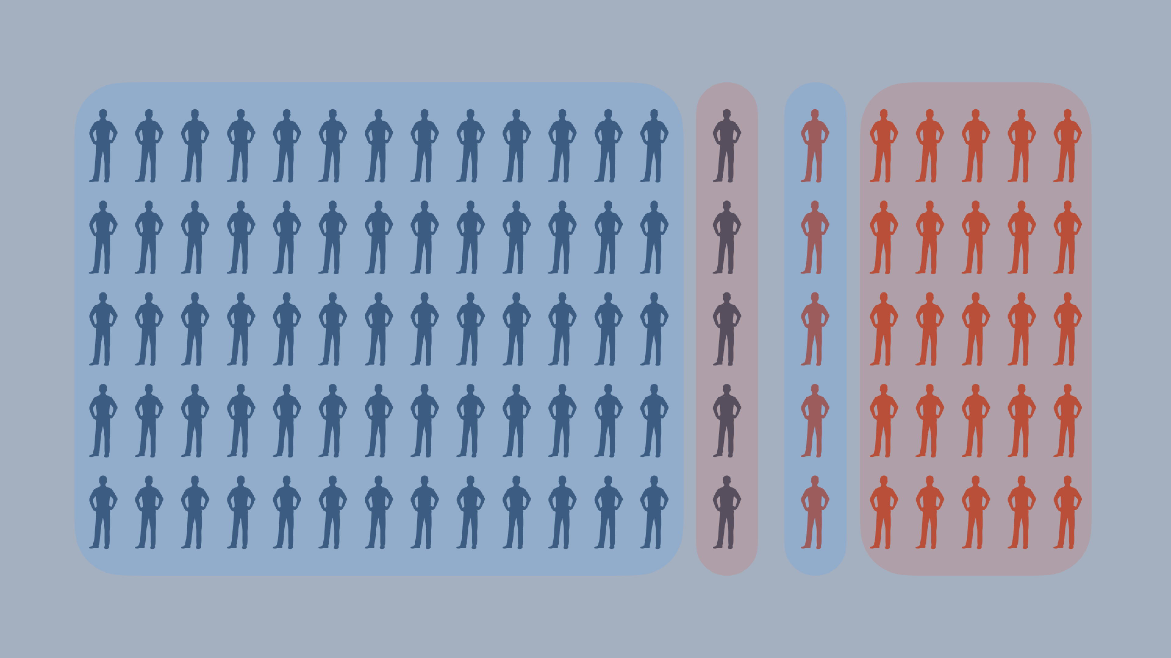
This graphic allows us to see where our model has classified positive and negative instances correctly and incorrectly—we won't worry about the proportions of true and false positives and negatives for now. This approach also allows us to use the initial four variables to define additional metrics that can help us to understand the performance of our model.

Let's define some key terms, all of which are based on the original confusion matrix:

Name	Label	Definition	Formal Definition
Actual Positives	P	The number of data points in the positive class, regardless of whether they were predicted correctly or incorrectly.	P = TP + FN
Actual Negatives	N	The number of data points in the negative class, regardless of whether they were predicted correctly or incorrectly.	N = TN + FP
Accuracy	ACC	The proportion of data points that were correctly predicted from the entire dataset.	ACC = (TP + TN) / (P + N)
Precision (or Positive Predictive Value)	Precision or PPV	The proportion of data points that were predicted to be in the positive class that were actually in the positive class.	PPV = TP / (TP + FP)
Recall (or True Positive Rate, or Sensitivity)	Recall or TPR	The proportion of data points in the positive class that were correctly predicted.	TPR = TP / P
False Positive Rate	FPR	The proportion of data points in the negative class that were incorrectly predicted.	FPR = FP / N

Table 2: A partial list of performance metrics

List of Metrics

There are many more performance metrics that can be extracted from a confusion matrix. We focus on the above ones simply because they are the ones needed for understanding some of the key concepts we discuss later on in this section.

The following table from (Ruf and Detyniecki, 2019)³ is a helpful reference for the most common metrics, and their paper is also an excellent resource in general.

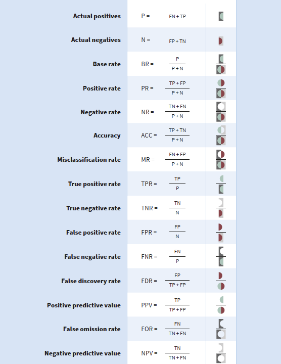
We have already looked at the first three terms from Table 1. Let's now look at Precision and Recall.

To get a general understanding of the two terms, consider the following image.

Here, the objective of the two fishing boats is to catch as many fish as possible. We can think of catching a fish as our positive class.

The "model" used by the boat on the left (i.e. the fishing rod) is very precise—it catches some of the fish (i.e. true positives), but not all of them, and it does not produce a lot of by-catch (e.g. false positives).

The "model" used by the boat on the right, however, has good recall—it catches (almost) all of the fish (i.e. true positives), but it also produces a lot of by-catch in the process (e.g. false positives).

This analogy is useful because it allows us to understand the trade-off between precision and recall. As we raise the classifier's boundary (i.e. increase the size of the net), we will increase the number of true positives for our model (or minimise the number of false negatives). However, in doing so, we will also increase the number of false positives.

But, if we lower the boundary (i.e. decrease the size of the net), we return to a situation where we have a higher number of false negatives but a lower number of false positives.

This is known as the precision-recall trade-off, and it brings us to our next statistical fairness issue.

Statistical Fairness Issue #2: The Precision-Recall Trade-off

This issue of where to "draw" the boundary for our classifier is a common one in machine learning, and the choice is in part a value-laden one. Both precision and recall are trying to maximise the number of true positives, but they also try to combine this objective with the further goal of minimising the number of false positives and false negatives, respectively.

Metric	Measures	What it Optimises
Precision	TP / (TP + FP)	Lower Rate of False Positives
Recall	TP / (TP + FN)	Lower Rate of False Negatives

Table 3: Comparison between precision and recall.

Another way to frame the intuition here is that precision is not as concerned with a higher number of false negatives, whereas recall is not as concerned with a higher number of false positives.

But, this translates into very different scenarios in the real world.

In our running example, a model with high precision will result in a higher rate of false negatives, which means that some patients may not receive treatment when they need it. In contrast, a model with high recall will capture more of these patients but some patients who do not need to be sent for further tests may have their time wasted and receive unsettling news.

In general, therefore, a high recall value is typically preferred because we generally deem the harm caused by a false positive to be less than the harm caused by a false negative. But this is not always the case—recall (pun intended) our example of the fishing boat, where minimising the amount of by-catch may be more important to ensure sustainable fishing practices.

The following quotation is helpful in understanding this trade-off:

"A general rule is that when the consequences of a positive prediction have a negative, punitive impact on the individual, the emphasis with respect to fairness often is on precision. When the result is rather beneficial in the sense that the individuals are provided help they would otherwise forgo, fairness is often more sensitive to recall." -- Ruf and Detyniecki (2021)

F0.5, F1, and F2 Scores

In machine learning, there is another approach to measuring accuracy that combines precision and recall into a single metric, known as the `F1` score.
The `F1` score is the harmonic mean of precision and recall, and is defined formally as follows:

$$
F1 = 2 \times \frac{Precision \times Recall}{Precision + Recall}
$$

A high F1 score means that the model has both high precision and high recall, and it balances the contribution of these two metrics such that they have equal weight.

However, as we have already seen, there are many real-world applications where either precision or recall may be more important goals.
In such cases, there are two variants of the F1 score that place different levels of emphasis on precision and recall: the F0.5 score (which favours precision), and the F2 score (which favours recall):

$$
F0.5 = (1 + 0.5^2) \times \frac{Precision \times Recall}{0.5^2 \times Precision + Recall}
$$

$$
F2 = (1 + 2^2) \times \frac{Precision \times Recall}{2^2 \times Precision + Recall}
$$

Note the addition of what is known as the `beta` parameter in the F0.5 and F2 scores, which is used to control the relative weight of precision and recall.
We do not discuss these variants in significant detail here, but [this article](https://machinelearningmastery.com/fbeta-measure-for-machine-learning/) provides a helpful introduction to the various scores, how to derive them, and shows how to use them in practice with code examples in Python.

So far, we have been treating our sample of patients as a homogeneous group. That is, we haven't considered whether there are different subgroups of patients that can be identified based on relevant characteristics (e.g. age, sex, race, etc.). This is a big gap from the perspective of fairness, but addressing it requires us to add some further complexity to our running example.

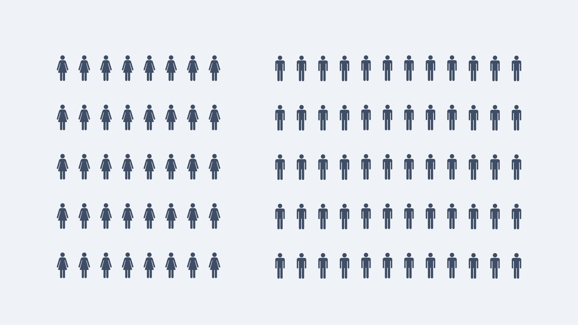
Therefore, let's assume that our 100 patients are now split according to their sex, and we have the following distribution.

Graphic showing a population of one hundred people, divided into forty females and 60 males.

With this update to our example, we need to return to our confusion matrix once more and consider how this new information alters our understanding of the performance of our model. Let's pretend that the performance of our model is as follows:

	Predicted Positive	Predicted Negative	Class Total
Actual Positive	10	10	20
Actual Negative	2	38	40

Table 4: Confusion Matrix for Females.

	Predicted Positive	Predicted Negative	Class Total
Actual Positive	7	6	13
Actual Negative	22	5	27

Table 5: Confusion Matrix for Males.

Again, we can represent this visually:

Graphic showing the outcome of a classification task for a population of one hundred people, divided into forty females and 60 males. The figures in red represent people who have the disease and the figures in blue represent healthy people. The red shading represents the people the model (correctly or incorrectly) classified as sick, while the blue shading is the analogous for healthy predictions..

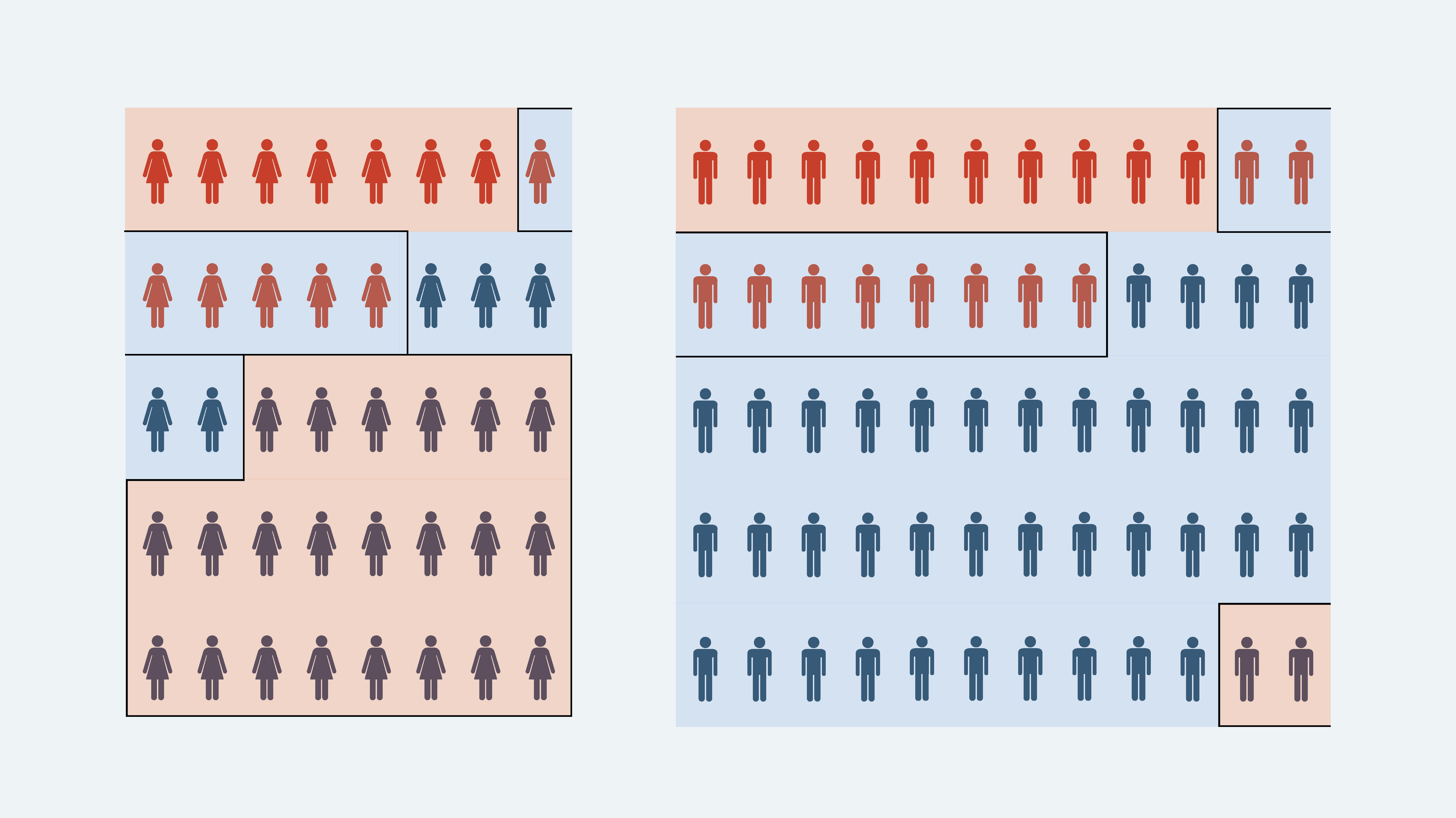
Let's now calculate some of the performance metrics for these two confusion matrices and show them side by side:

Metric	Male	Female
True Positive Rate (TP / P)	0.5	0.5
False Positive Rate (FP / N)	0.05	0.8
True Negative Rate (TN / N)	0.95	0.2
False Negative Rate (FN / P)	0.5	0.5
Accuracy ((TP + TN) / (P + N))	0.8	0.3
Precision (TP / (TP + FP))	0.8	0.24
Recall (TP / (TP + FN))	0.5	0.5

Table 6: Metrics for Females and Males.

As you can see, there is variation in the performance of our model across the two subgroups in a number of categories. Although recall is the same for the two groups, the accuracy and precision of the models differ significantly because of the higher number of false positives for females.

Translated into practical terms, this means our current model will send a large proportion of non-sick female patients for further tests or treatment, because it incorrectly classifies them as sick.

What can we do about this?

A few options include:

• Collecting more data and improving the representativeness of the dataset to see if we can reduce the class imbalance
• Altering the decision threshold for the model to see if the precision-recall trade-off can be improved, perhaps by using the F-score as a guide
• Oversampling from the minority group to rebalance the classes

There are myriad pros and cons to these approaches. But before we even consider such approaches, we need to touch upon another important statistical fairness issue: the base-rate.

Statistical Fairness Issue #3: Variation in Base Rate

First, the base rate is just the number of positive cases divided by the total number of cases:

\[ BR = \frac{P}{P+N} \]

In the previous example, the base rate was the same for both subgroups. But this is often not the case in real-world datasets, especially in healthcare where the prevalence of a disease can vary drastically between different subgroups (e.g. affecting elderly patients more than young patients).

So, let's now change the base rate and review how this affects our model.

	Predicted Positive	Predicted Negative	Class Total
Actual Positive	10	10	20
Actual Negative	2	38	40

Table 7: New Confusion Matrix for Females

	Predicted Positive	Predicted Negative	Class Total
Actual Positive	18	9	27
Actual Negative	11	2	13

Table 8: New Confusion Matrix for Males

Let's now calculate some of the performance metrics for these two confusion matrices and show them side by side:

Metric	Male	Female
Base Rate (P / P + N)	0.33	0.68
True Positive Rate (TP / P)	0.5	0.67
False Positive Rate (FP / N)	0.05	0.85
True Negative Rate (TN / N)	0.95	0.15
False Negative Rate (FN / P)	0.5	0.33
Accuracy ((TP + TN) / (P + N))	0.8	0.5
Precision (TP / (TP + FP))	0.8	0.62
Recall (TP / (TP + FN))	0.5	0.67

Table 9: New Metrics for Females and Males

So, now we have a situation where the likelihood of having the disease is higher for females (i.e. a base rate of 0.68 for females and a base rate of 0.33 for males), and they are under-represented in our dataset. Furthermore, although there is an improvement from the previous set of metrics, this hypothetical model still has higher levels of performance for males who are over-represented in the dataset and less likely to have the disease.

Intuitively, this is not a fair model. But can we be more precise in saying why?

A first pass would appeal to moral and legalistic notions of non-discrimination and equality. We have not spoken about which features our model is using in this running example, but let's pretend that the project team did not use the sex of the patients as features for their model. Rather, they kept this data back solely as a means for evaluating the fairness of the model.

Perhaps their reason for this decision was that they were motivated by a conception of fairness-as-blindness, where the model should not be able to discriminate against any protected characteristic.⁴ However, despite not using sex when training their model, the model still ended up discriminating against female patients. Because of the variation in base rate, perhaps having a model that took account of sex would have been preferable, as it would have allowed the model to condition on the presence of this variable when forming predictions.

In legal terms, the above decision of the project team would give rise to an instance of 'indirect discrimination', whether intentional or not. Indirect discrimination means that some rule, policy, practice, or in this case an 'algorithm', appears to be neutral with respect to how it treats different groups, but has a disproportionate impact on a protected group.

The notion of a protected group or characteristic is a helpful one in fair data science and AI, because it allows us to bring additional precision to our discussion and helps us identify different types of fairness (and unfairness) as we will see in the next section.

What is a protected group?

As defined in the UK's Equality Act 2010⁵, it is against the law to discriminate against anyone because of the following protected characteristics:

• age
• gender reassignment
• being married or in a civil partnership
• being pregnant or on maternity leave
• disability
• race including colour, nationality, ethnic or national origin
• religion or belief
• sex
• sexual orientation

When we refer to a 'protected group', we are referring to a group whose members share one of these characteristic.

However the concept of a 'protected characteristic' is not without its problems. For instance, poverty is not a protected characteristic in the UK, but it is a well-known predictor of poor health outcomes. As such, if a model is trained on data that includes a proxy for poverty (e.g. the area in which a patient lives), it may end up discriminating against patients from poorer areas, but there would be little legal recourse for the patients to seek redress.

What is a proxy?

The term 'proxy' in data science is used to refer to the situation where one feature (A) is highly correlated with another feature (B). That is, A is a proxy for B, such that even if we do not use B as a feature in our model, the presence of A in our dataset could still capture the statistical effects of B.

Your activity on social media, for example, can serve as a proxy for many different characteristics, including your age, political beliefs, and sexual orientation, and has been used by various companies (with dubious ethical standards) to infer these characteristics where they are not directly provided by the user.

Therefore, although we will refer to 'protected characteristics' in the remainder of this discussion, it is worth keeping in mind whether the moral scope of this term is adequately captured by the legal definitions.

Statistical Fairness (or, Non-Discrimination) Criteria

If we are to choose responsible methods for addressing inequalities in model performance, such as the ones we have just discussed, we need to be able to precisely identify how and where the model is failing to be fair.

Researchers have put forward dozens of different statistical criteria that all seek to capture different intuitions about what is fair. However, in their excellent book on fair machine learning, Barocas et al. (2019)⁴ show how these different criteria can be grouped together, forming three over-arching criteria of non-discrimination that all bear on the relationship between the model's performance across sub-groups. These three criteria formally define a variety of 'group-level' fairness criteria, which we can then use to determine targets for our model to achieve or constraints to impose during the development of the model.

Individual vs. Group Fairness

This section is concerned with group-level fairness criteria, and the introduction of a tool that helps to decide between different definitions of group fairness. Group-level fairness only provides assurance that the average member of a (protected, marginalised or vulnerable) group will be treated fairly. No guarantees are provided to individuals.

However, it is worth noting that there are also individual-level fairness criteria, which are concerned with the fairness of the model's predictions between individuals. For instance, if two individuals are similar in terms of relevant characteristics, then they should have similar chances of being classified as positive or negative.

See (Mehrabi, 2019) for a survey of bias and fairness in machine learning that includes a discussion of individual-level fairness criteria.⁶

To understand these criteria, we first need to define a few key variables:

• \(Y\) is the outcome variable, which is the variable we are trying to predict.
• \(\hat{Y}\) is the prediction of the model.
• \(A\) is the protected characteristic. For simplicity, we will assume there is only one relevant protected characteristic \(A\), and that individuals either have it or do not.

Now, we can define the three criteria as follows:

• Independence: the protected characteristic \(A\) is unconditionally independent of the model's predictions \(\hat{Y}\)
• Separation: \(A\) is conditionally independent of the model's predictions \(\hat{Y}\), given the true outcome \(Y\)
• Sufficiency: \(A\) is conditionally independent of the true outcome \(Y\), given the model's predictions \(\hat{Y}\)

These formal criteria can be a little hard to understand, and moreover, it can be hard to see why meeting them would be a good thing from the perspective of fairness.

However, Barocas et al. (2019) explain that meeting each of these criteria equalises one of the following across all groups:

• Acceptance rate: the acceptance rate of the model, i.e. the proportion of individuals who are predicted to have the outcome, should be equal across all groups.
• Outcome frequency: the distribution of the outcome variable, i.e. the proportion of individuals who have the outcome, should be equal across all groups.
• Error rates: the error rates of the model, i.e. the distribution of false negatives and false positives, should be equal across all groups.

There is not a simple one-to-one mapping that exist between the criteria and these three rates/frequencies, because for each of the three criteria there are myriad compatible definitions of fairness that aim at different rates/frequencies. For instance, Ruf and Detyniecki provide the following list of compatible definitions of fairness for each of the three criteria.³

Criteria	Compatible definitions of fairness
Independence	Demographic parity Conditional statistical parity Equal selection parity
Separation	Equalized odds Equalised opportunity Predictive equality Balance
Sufficiency	Conditional use accuracy equality Predictive Parity Calibration

Table 10: Various Definitions of Statistical Fairness grouped by three Main Criteria.

It can quickly become overwhelming to try to decide which of these criteria to aim for, which type of fairness is most important to your project, and which of the many definitions of fairness to use for each criteria. Fortunately, there is a tool that can help us decide which of these criteria to aim for based on specific properties that may be present in our data or project.

The Fairness Compass: A Tool for Choosing Fairness Criteria

The Fairness Compass is a tool created by Ruf and Detyniecki (2021) to help researchers and developers choose between the three fairness criteria we have just discussed. It allows a project team to ask a series of questions related to their data and project, which can narrow down the permissible fairness criteria.

Some of these questions include the following:

• Is there a policy in place that requires the project to go beyond the mere equal treatment of different groups to proactively reducing existing inequalities by boosting underprivileged groups (e.g. through affirmative action)?
• Are there equal base rates of the outcome variable across groups?
• Is your conception of fairness sensitive to a particular error type, such that you need to optimise for precision or recall?

These questions are helpfully presented as a decision tree algorithm, terminating in the three fairness criteria discussed above, as well as a variety of specific implementations of each criteria.

Graphic showing the Fairness Compass Tool developed by Ruf & Detyniecki (2021).

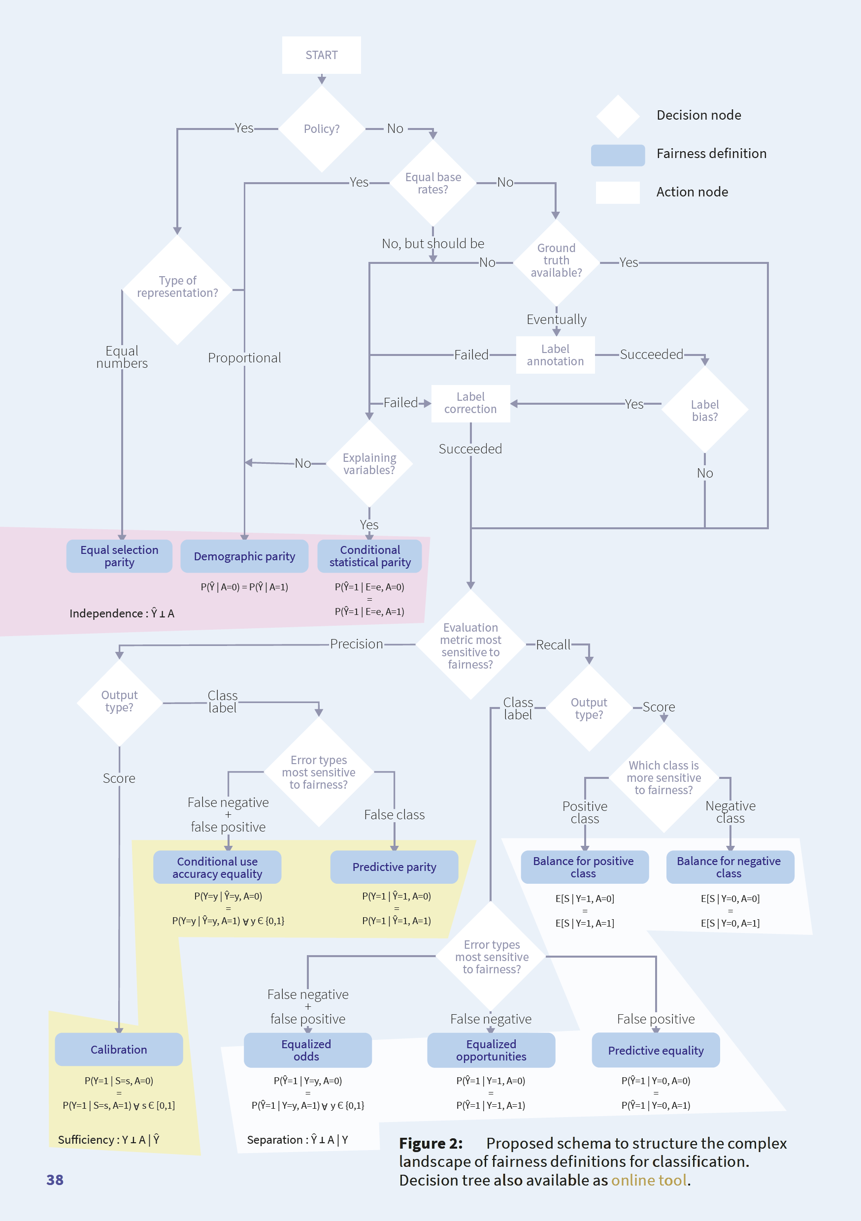
Interactive Tool and Paper

We are not going to go through the entire tool here. Rather, an interactive version is available, which has helpful tooltips to explain the questions and the options available to the user. We also highly recommend reading the accompanying paper.

One of the questions raised by the tool, however, brings us to our final statistical fairness issue: whether we have access to the ground truth.

Statistical Fairness Issue #4: Ground Truth

The final assumption made in our running example that we will discuss is the existence of a ground truth label for each of our data points. In the case of the medical diagnosis example, this would be the presence of a disease, confirmed via some medical test, which we previously referred to as \(Y\).

To effectively evaluate the performance of a model, we need to know the true value of the outcome variable for each data point \(Y\) and how far the model's predictions \(\hat{Y}\) are from this true value.

In the case of medical diagnosis, confidence in our ground truth may be achieved through secondary testing. For instance, if we know that an initial diagnostic test (responsible for generating our training data) is good but not perfect, then we can use a second test that has higher precision to confirm an initial diagnosis and reduce the number of false positives. In cases where the secondary test is more invasive or expensive, this may be the best option.

But what happens when there is no such procedure?

Mental health diagnosis is a good example of this. There is a huge literature on whether the procedures and labels we use to diagnose patients with mental health conditions are valid. For instance, how valid and reliable are the psychometric tests used during assessment or diagnosis (e.g. PHQ-9), given they rely on self-reporting? Are such tests able to accommodate intercultural variation in the way that mental health conditions are expressed and understood? Are constructs like depression or anxiety able to adequately capture the biopsychosocial complexity of mental health conditions?

None of these questions should be misconstrued as undermining the existence or lived experience of mental health conditions. But they do raise questions about the use of such labels as the "ground truth" in the context of machine learning classification. Perhaps the labels are imperfect proxies for a more complex and unobservable phenomenon that is difficult to measure. But, if so, should we be using them as the basis for training and evaluating our models, and what further limitations does this place on our ability to reliably measure the fairness of our models?

Unfortunately, there is no simple answer to such a question, as it is inherently entangled within the context in which the model is being used.

The Problem with Missing Ground Truth: An Infamous Case Study

A now infamous case study published by Obermeyer et al. (2019), explored and dissected an algorithm that contained racial bias due to its use of predicted `health care cost` as a proxy for the actual target variable `illness` (or `healthcare need`).

The indirect consequence of this design choice was that the algorithm systematically underestimated the healthcare needs of Black patients, while overestimating the healthcare needs of White patients. 
The result was significant disparities in care between the two groups.

As the authors go on to explain, this issue arises in part due to systematic biases in American healthcare (e.g. barriers to accessing healthcare, or implicit biases of healthcare professionals), which become encoded in the proxy variable `healthcare cost`.

As the authors note:

> We suggest that the choice of convenient, seemingly effective proxies for ground truth can be an important source of algorithmic bias in many contexts.

This section has explored several concepts and issues with statistical fairness. However, we have barely scratched the surface of the topic.

Nevertheless, we have seen enough to understand some of the limitations of the statistical fairness criteria we have discussed, and also introduce some practical metrics and tools that can be applied to help improve the fairness of our models in terms of non-discrimination and equal opportunity.

In the final section of this module, we are going to look at why some of these issues arise in the first place, by exploring the multifaceted concept of 'bias'.

---

1. Nielsen, A. (2020). Practical fairness. O'Reilly Media. ↩

2. Powles, J., & Nissembaum, H. (2018, December 7). The seductive diversion of ‘solving’ bias in artificial intelligence. Medium. https://onezero.medium.com/the-seductive-diversion-of-solving-bias-in-artificial-intelligence-890df5e5ef53 ↩

3. Ruf, B., & Detyniecki, M. (2021). Towards the right kind of fairness in AI. https://axa-rev-research.github.io/static/AXA_FairnessCompass-English.pdf ↩↩

4. Barocas, S., Hardt, M., & Narayanan, A. (2019). Fairness and machine learning: Limitations and opportunities. fairmlbook.org http://www.fairmlbook.org ↩↩

5. See: https://www.gov.uk/discrimination-your-rights ↩

6. Mehrabi, N., Morstatter, F., Saxena, N., Lerman, K., & Galstyan, A. (2019). A Survey on Bias and Fairness in Machine Learning. ArXiv:1908.09635 [Cs]. http://arxiv.org/abs/1908.09635 ↩