1.0 Introduction to Python#

Estimated time for this notebook: 10 minutes

1.0.1 Why write programs for research?#

Programs are a rigorous way of describing data analysis for other researchers, as well as for computers.

Not just labour saving
Scripted research can be tested and reproduced

Sensible Input - Reasonable Output#

Computational research suffers from people assuming each other’s data manipulation is correct. By sharing code, which is much more easy for a non-author to understand than a spreadsheet, we can avoid the “SIRO” problem. The old saw “Garbage in Garbage out” is not the real problem for science:

Sensible input
Reasonable output

Why write software to manage your data and plots?#

We can use programs for our entire research pipeline. Not just big scientific simulation codes, but also the small scripts which we use to tidy up data and produce plots. This should be code, so that the whole research pipeline is recorded for reproducibility. Data manipulation in spreadsheets is much harder to share or check. There are many data analysis examples out there, like the on the software carpentry site.

1.0.2 Why Python?#

Why teach Python?#

In this first session, we will introduce Python.
This course is about programming for data analysis and visualisation in research.
It’s not mainly about Python.
But we have to use some language.

Why Python?#

Python is quick to program in
Python is popular in research, and has lots of libraries for science
Python interfaces well with faster languages
Python is free, so you’ll never have a problem getting hold of it, wherever you go.

1.0.3 Many kinds of Python#

The Jupyter Notebook#

The easiest way to get started using Python, and one that is commonly used for exploratory research, is the Jupyter Notebook.

In the notebook, you can easily mix code with discussion and commentary. You can also mix code with the results of that code, such as graphs and other data visualisations.

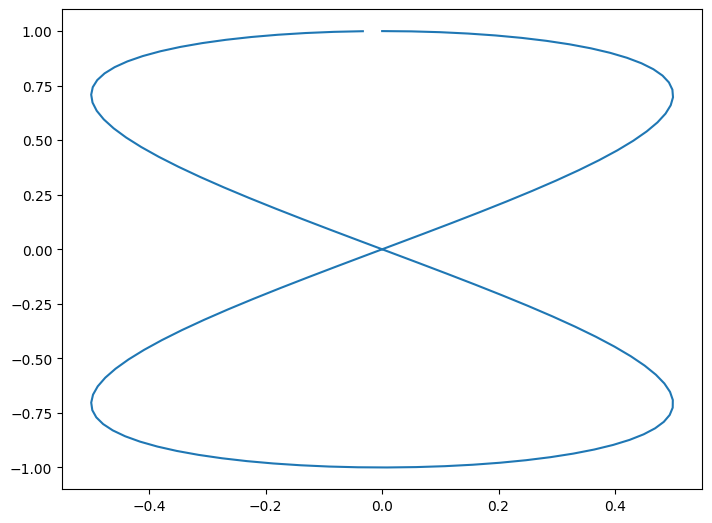
# Make plot
%matplotlib inline
import math

import matplotlib.pyplot as plt
import numpy as np

theta = np.arange(0, 4 * math.pi, 0.1)
eight = plt.figure()
axes = eight.add_axes([0, 0, 1, 1])
axes.plot(0.5 * np.sin(theta), np.cos(theta / 2))

[<matplotlib.lines.Line2D at 0x7f9d3cc90790>]

../_images/01_00_introduction_to_python_17_1.png

We’re going to be mainly working in the Jupyter notebook in this course. To get hold of a copy of the notebook, follow the setup instructions shown on the course website.

Jupyter notebooks consist of discussion cells, referred to as “markdown cells”, and “code cells”, which contain Python. This document has been created using Jupyter notebook, and this very cell is a Markdown Cell.

print("This cell is a code cell")

This cell is a code cell

Code cell inputs are numbered, and show the output below.

Markdown cells contain text which uses a simple format to achive pretty layout, for example, to obtain:

bold, italic

Bullet

Quote

We write:

**bold**, *italic*

* Bullet

> Quote

See the Markdown documentation at This Hyperlink

Typing code in the notebook#

When working with the notebook, you can either be in a cell, typing its contents, or outside cells, moving around the notebook.

When in a cell, press escape to leave it. When moving around outside cells, press return to enter.
Outside a cell:
- Use arrow keys to move around.
- Press b to add a new cell below the cursor.
- Press m to turn a cell from code mode to markdown mode.
- Press shift+enter to calculate the code in the block.
- Press h to see a list of useful keys in the notebook.
Inside a cell:
- Press tab to suggest completions of variables. (Try it!)

Supplementary material: Learn more about Jupyter notebooks.

Python at the command line#

More experience Python users tend to prefer working in a “command line environment”. You can find out more about this by attending a “Software Carpentry” or similar workshop, which introduce the skills needed for computationally based research.

%%bash
# Above line tells Python to execute this cell as *shell code*
# not Python, as if we were in a command line
# This is called a 'cell magic'

python -c "print(2 * 4)"

Python scripts#

When your code gets more complicated, you’ll want to be able to write your own full programs in Python, which can be run just like any other program on your computer. Here are some examples:

%%bash
echo "print(2 * 4)" > eight.py
python eight.py

We can make the script directly executable (on Linux or Mac) by inserting a shebang and setting the permissions to execute.

%%writefile fourteen.py
#! /usr/bin/env python
print(2 * 7)

Overwriting fourteen.py

%%bash
chmod u+x fourteen.py
./fourteen.py

Python Libraries#

We can write our own python libraries, called modules which we can import into the notebook and invoke:

%%writefile draw_eight.py
# Above line tells the notebook to treat the rest of this
# cell as content for a file on disk.
import math
import numpy as np
import matplotlib.pyplot as plt


def make_figure():
    theta = np.arange(0, 4 * math.pi, 0.1)
    eight = plt.figure()
    axes = eight.add_axes([0, 0, 1, 1])
    axes.plot(0.5 * np.sin(theta), np.cos(theta / 2))
    return eight

Overwriting draw_eight.py

In a real example, we could edit the file on disk using a program such as Atom or VS code.

import draw_eight  # Load the library file we just wrote to disk

image = draw_eight.make_figure()

../_images/01_00_introduction_to_python_40_0.png

There is a huge variety of available packages to do pretty much anything. For instance, try import antigravity.

The %% at the beginning of a cell is called magics. There’s a large list of them available and you can create your own.

Research Software Engineering with Python

1.0 Introduction to Python

Contents