3.6 The Boids!
Contents
3.6 The Boids!#
Estimated time to complete this notebook: 45 minutes.
⚠️ Warning: Advanced Topic! ⚠️
Our earlier discussion of NumPy was very theoretical, but let’s go through a practical example, and see how powerful NumPy can be.
Note this is more a showcase of what you can do with numpy than an exhaustive notebook to work through
3.6.1 Flocking#
The aggregate motion of a flock of birds, a herd of land animals, or a school of fish is a beautiful and familiar part of the natural world… The aggregate motion of the simulated flock is created by a distributed behavioral model much like that at work in a natural flock; the birds choose their own course. Each simulated bird is implemented as an independent actor that navigates according to its local perception of the dynamic environment, the laws of simulated physics that rule its motion, and a set of behaviors programmed into it… The aggregate motion of the simulated flock is the result of the dense interaction of the relatively simple behaviors of the individual simulated birds.
– Craig W. Reynolds, “Flocks, Herds, and Schools: A Distributed Behavioral Model”, Computer Graphics 21 4 1987, pp 25-34
We will demonstrate an algorithm to simulate flocking behaviour in numpy. The simulation consists of a set of individual bird-like objects that we will call ‘boids’ following the nomenclature of the original paper for more details.
Collision Avoidance: avoid collisions with nearby flockmates
Velocity Matching: attempt to match velocity with nearby flockmates
Flock Centering: attempt to stay close to nearby flockmates
3.6.2 Setting up the Boids#
Our boids will each have an x velocity and a y velocity, and an x position and a y position.
We’ll build this up in NumPy notation, and eventually, have an animated simulation of our flying boids.
import numpy as np
Let’s start with simple flying in a straight line.
Our positions, for each of our N boids, will be an array, shape \(2 \times N\), with the x positions in the first row, and y positions in the second row.
boid_count = 10
We’ll want to be able to seed our Boids in a random position.
We’d better define the edges of our simulation area:
limits = np.array([2000, 2000])
positions = np.random.rand(2, boid_count) * limits[:, np.newaxis]
positions
array([[1469.30273805, 1974.20093305, 466.31181046, 974.18910549,
88.93015656, 437.19012488, 1096.64793516, 1374.47388504,
976.09255964, 306.61982305],
[1574.08191225, 446.65970454, 1281.42970812, 1085.79252945,
1894.15030894, 951.18768334, 108.86417594, 1020.29384278,
870.54477731, 116.85914325]])
positions.shape
(2, 10)
We used broadcasting with np.newaxis to apply our upper limit to each boid. rand gives us a random number between 0 and 1.
We multiply by our limits to get a number up to that limit.
limits[:, np.newaxis]
array([[2000],
[2000]])
limits[:, np.newaxis].shape
(2, 1)
np.random.rand(2, boid_count).shape
(2, 10)
So we multiply a \(2\times1\) array by a \(2 \times 10\) array – and get a \(2\times 10\) array.
Let’s put that in a function:
def new_flock(count, lower_limits, upper_limits):
width = upper_limits - lower_limits
return lower_limits[:, np.newaxis] + np.random.rand(2, count) * width[:, np.newaxis]
For example, let’s assume that we want our initial positions to vary between 100 and 200 in the x axis, and 900 and 1100 in the y axis. We can generate random positions within these constraints with:
positions = new_flock(boid_count, np.array([100, 900]), np.array([200, 1100]))
But each boid will also need a starting velocity. Let’s make these random too:
We can reuse the new_flock function defined above, since we’re again essentially just generating random numbers from given limits.
This saves us some code, but keep in mind that using a function for something other than what its name indicates can become confusing!
Here, we will let the initial x velocities range over \([0, 10]\) and the y velocities over \([-20, 20]\).
velocities = new_flock(boid_count, np.array([0, -20]), np.array([10, 20]))
velocities
array([[ 6.11741937, 8.46349346, 4.39221673, 7.99412569,
0.66413959, 5.85312869, 5.88237949, 5.51073276,
9.42240838, 0.030474 ],
[ -2.39277863, 0.92740242, -1.98751009, 12.17621129,
6.0136092 , -3.93489978, 8.90194992, -4.95790977,
-8.86321783, -19.56530663]])
3.6.3 Flying in a Straight Line#
Now we see the real amazingness of NumPy: if we want to move our whole flock according to
\(\delta_x = \delta_t \cdot \frac{dv}{dt}\)
we just do:
positions += velocities
3.6.4 Matplotlib Animations#
So now we can animate our Boids using the matplotlib animation tools All we have to do is import the relevant libraries:
from matplotlib import animation
from matplotlib import pyplot as plt
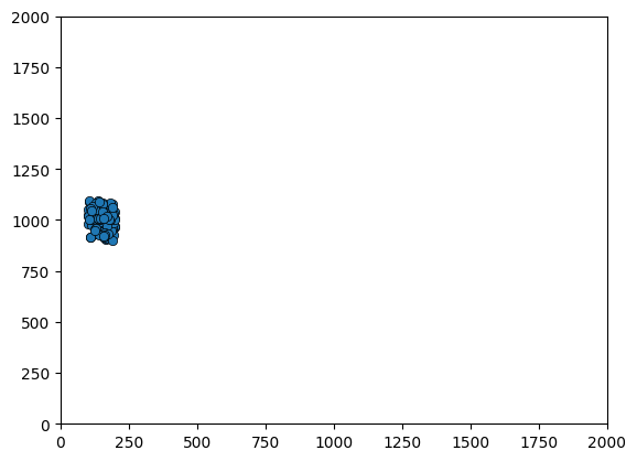
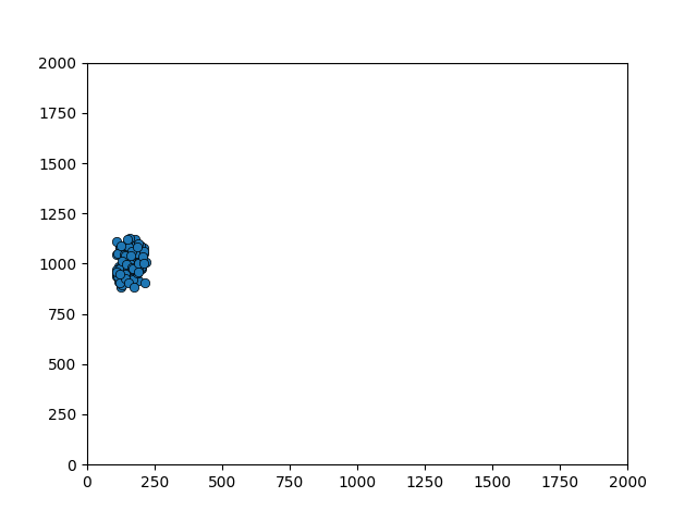
Then, we make a static plot, showing our first frame:
# create a simple plot
# initial x position in [100, 200], initial y position in [900, 1100]
# initial x velocity in [0, 10], initial y velocity in [-20, 20]
positions = new_flock(100, np.array([100, 900]), np.array([200, 1100]))
velocities = new_flock(100, np.array([0, -20]), np.array([10, 20]))
figure = plt.figure()
axes = plt.axes(xlim=(0, limits[0]), ylim=(0, limits[1]))
scatter = axes.scatter(
positions[0, :], positions[1, :], marker="o", edgecolor="k", lw=0.5
)
scatter
<matplotlib.collections.PathCollection at 0x7fcb4c1fbc70>
Then, we define a function which updates the figure for each timestep
def update_boids(positions, velocities):
positions += velocities
def animate(frame):
update_boids(positions, velocities)
scatter.set_offsets(positions.transpose())
Call FuncAnimation, and specify how many frames we want:
anim = animation.FuncAnimation(figure, animate, frames=50, interval=50)
Save out the figure:
positions = new_flock(100, np.array([100, 900]), np.array([200, 1100]))
velocities = new_flock(100, np.array([0, -20]), np.array([10, 20]))
anim.save("boids_1.gif")
And download the saved animation.
You can even view the results directly in the notebook.
from IPython.display import HTML
positions = new_flock(100, np.array([100, 900]), np.array([200, 1100]))
velocities = new_flock(100, np.array([0, -20]), np.array([10, 20]))
HTML(anim.to_jshtml())
3.6.5 Extended content: The Boids!#
The examples given below are examples of how to use numpy to efficiently apply equations to arrays. here are many potential ways to do such things, and this is intended as a showcase of numpy’s versatility rather than a prescribed set of rules.
3.6.5.0 Fly towards the middle#
Boids try to fly towards the middle:
positions = new_flock(4, np.array([100, 900]), np.array([200, 1100]))
velocities = new_flock(4, np.array([0, -20]), np.array([10, 20]))
positions
array([[ 118.24104664, 110.1167461 , 163.28688425, 155.09459038],
[ 916.71730853, 941.53723637, 1018.60095439, 1016.78246459]])
velocities
array([[ 2.81106366, 4.82654397, 6.59162093, 9.06034214],
[-15.99577591, 3.26285871, -3.33845727, -12.93699006]])
middle = np.mean(positions, 1)
middle
array([136.68481684, 973.40949097])
direction_to_middle = positions - middle[:, np.newaxis]
direction_to_middle
array([[-18.4437702 , -26.56807074, 26.60206741, 18.40977354],
[-56.69218244, -31.8722546 , 45.19146342, 43.37297362]])
This is easier and faster than:
for boid in boids:
for dimension in [0, 1]:
direction_to_middle[dimension][boid] = positions[dimension][boid] - middle[dimension]
move_to_middle_strength = 0.01
velocities = velocities - direction_to_middle * move_to_middle_strength
Let’s update our function, and animate that:
def update_boids(positions, velocities):
move_to_middle_strength = 0.01
middle = np.mean(positions, 1)
direction_to_middle = positions - middle[:, np.newaxis]
velocities -= direction_to_middle * move_to_middle_strength
positions += velocities
def animate(frame):
update_boids(positions, velocities)
scatter.set_offsets(positions.transpose())
anim = animation.FuncAnimation(figure, animate, frames=50, interval=50)
positions = new_flock(100, np.array([100, 900]), np.array([200, 1100]))
velocities = new_flock(100, np.array([0, -20]), np.array([10, 20]))
HTML(anim.to_jshtml())
3.6.5.1 Avoiding collisions#
We’ll want to add our other flocking rules to the behaviour of the Boids.
We’ll need a matrix giving the distances between each boid. This should be \(N \times N\).
positions = new_flock(4, np.array([100, 900]), np.array([200, 1100]))
velocities = new_flock(4, np.array([0, -20]), np.array([10, 20]))
We might think that we need to do the X-distances and Y-distances separately:
xpos = positions[0, :]
xsep_matrix = xpos[:, np.newaxis] - xpos[np.newaxis, :]
xsep_matrix.shape
(4, 4)
xsep_matrix
array([[ 0. , 18.95947862, 44.98709169, 28.08217295],
[-18.95947862, 0. , 26.02761307, 9.12269432],
[-44.98709169, -26.02761307, 0. , -16.90491874],
[-28.08217295, -9.12269432, 16.90491874, 0. ]])
But in NumPy we can be cleverer than that, and make a \(2 \times N \times N\) matrix of separations:
separations = positions[:, np.newaxis, :] - positions[:, :, np.newaxis]
separations.shape
(2, 4, 4)
And then we can get the sum-of-squares \(\delta_x^2 + \delta_y^2\) like this:
squared_displacements = separations * separations
square_distances = np.sum(squared_displacements, 0)
square_distances
array([[ 0. , 9071.45255165, 6701.17553731, 9495.03384416],
[9071.45255165, 0. , 1299.78871224, 83.22444082],
[6701.17553731, 1299.78871224, 0. , 906.64152621],
[9495.03384416, 83.22444082, 906.64152621, 0. ]])
Now we need to find boids that are too close:
alert_distance = 2000
close_boids = square_distances < alert_distance
close_boids
array([[ True, False, False, False],
[False, True, True, True],
[False, True, True, True],
[False, True, True, True]])
Find the direction distances only to those boids which are too close:
separations_if_close = np.copy(separations)
far_away = np.logical_not(close_boids)
Set x and y values in separations_if_close to zero if they are far away:
separations_if_close[0, :, :][far_away] = 0
separations_if_close[1, :, :][far_away] = 0
separations_if_close
array([[[ 0. , 0. , 0. , 0. ],
[ 0. , 0. , -26.02761307, -9.12269432],
[ 0. , 26.02761307, 0. , 16.90491874],
[ 0. , 9.12269432, -16.90491874, 0. ]],
[[ 0. , 0. , 0. , 0. ],
[ 0. , 0. , 24.94698519, 0.02981745],
[ 0. , -24.94698519, 0. , -24.91716775],
[ 0. , -0.02981745, 24.91716775, 0. ]]])
And fly away from them:
np.sum(separations_if_close, 2)
array([[ 0. , -35.15030739, 42.93253181, -7.78222442],
[ 0. , 24.97680264, -49.86415294, 24.8873503 ]])
velocities = velocities + np.sum(separations_if_close, 2)
Now we can update our animation:
def update_boids(positions, velocities):
move_to_middle_strength = 0.01
middle = np.mean(positions, 1)
direction_to_middle = positions - middle[:, np.newaxis]
velocities -= direction_to_middle * move_to_middle_strength
separations = positions[:, np.newaxis, :] - positions[:, :, np.newaxis]
squared_displacements = separations * separations
square_distances = np.sum(squared_displacements, 0)
alert_distance = 100
far_away = square_distances > alert_distance
separations_if_close = np.copy(separations)
separations_if_close[0, :, :][far_away] = 0
separations_if_close[1, :, :][far_away] = 0
velocities += np.sum(separations_if_close, 1)
positions += velocities
def animate(frame):
update_boids(positions, velocities)
scatter.set_offsets(positions.transpose())
anim = animation.FuncAnimation(figure, animate, frames=50, interval=50)
positions = new_flock(100, np.array([100, 900]), np.array([200, 1100]))
velocities = new_flock(100, np.array([0, -20]), np.array([10, 20]))
HTML(anim.to_jshtml())
3.6.5.2 Match speed with nearby boids#
This is pretty similar:
def update_boids(positions, velocities):
move_to_middle_strength = 0.01
middle = np.mean(positions, 1)
direction_to_middle = positions - middle[:, np.newaxis]
velocities -= direction_to_middle * move_to_middle_strength
separations = positions[:, np.newaxis, :] - positions[:, :, np.newaxis]
squared_displacements = separations * separations
square_distances = np.sum(squared_displacements, 0)
alert_distance = 100
far_away = square_distances > alert_distance
separations_if_close = np.copy(separations)
separations_if_close[0, :, :][far_away] = 0
separations_if_close[1, :, :][far_away] = 0
velocities += np.sum(separations_if_close, 1)
velocity_differences = velocities[:, np.newaxis, :] - velocities[:, :, np.newaxis]
formation_flying_distance = 10000
formation_flying_strength = 0.125
very_far = square_distances > formation_flying_distance
velocity_differences_if_close = np.copy(velocity_differences)
velocity_differences_if_close[0, :, :][very_far] = 0
velocity_differences_if_close[1, :, :][very_far] = 0
velocities -= np.mean(velocity_differences_if_close, 1) * formation_flying_strength
positions += velocities
def animate(frame):
update_boids(positions, velocities)
scatter.set_offsets(positions.transpose())
anim = animation.FuncAnimation(figure, animate, frames=200, interval=50)
positions = new_flock(100, np.array([100, 900]), np.array([200, 1100]))
velocities = new_flock(100, np.array([0, -20]), np.array([10, 20]))
HTML(anim.to_jshtml())
Hopefully the power of numpy should be pretty clear now.
This would be enormously slower and, I think, harder to understand using traditional lists.