3.4 NumPy
Contents
3.4 NumPy#
Estimated time to complete this notebook: 20 minutes
3.4.1 Limitations of Python Lists#
The normal Python List is just one dimensional. To make a matrix, we have to nest Python lists:
x = [list(range(5)) for N in range(5)]
x
[[0, 1, 2, 3, 4],
 [0, 1, 2, 3, 4],
 [0, 1, 2, 3, 4],
 [0, 1, 2, 3, 4],
 [0, 1, 2, 3, 4]]
x[2][2]
2
Applying an operation to every element is a pain:
x + 5
---------------------------------------------------------------------------
TypeError                                 Traceback (most recent call last)
Cell In[4], line 1
----> 1 x + 5

TypeError: can only concatenate list (not "int") to list
[[elem + 5 for elem in row] for row in x]
[[5, 6, 7, 8, 9],
 [5, 6, 7, 8, 9],
 [5, 6, 7, 8, 9],
 [5, 6, 7, 8, 9],
 [5, 6, 7, 8, 9]]
Common useful operations like transposing a matrix or reshaping a 10 by 10 matrix into a 20 by 5 matrix are not easy to code in raw Python lists.
3.4.2 The NumPy array#
NumPy’s array type represents a multidimensional matrix \(M_{i,j,k...n}\)
The NumPy array seems at first to be just like a list:
import numpy as np

my_array = np.array(range(5))
my_array
array([0, 1, 2, 3, 4])
my_array[2]
2
for element in my_array:
    print("Hello" * element)
Hello
HelloHello
HelloHelloHello
HelloHelloHelloHello
We can also see our first weakness of NumPy arrays versus Python lists:
my_array.append(4)
---------------------------------------------------------------------------
AttributeError                            Traceback (most recent call last)
Cell In[10], line 1
----> 1 my_array.append(4)

AttributeError: 'numpy.ndarray' object has no attribute 'append'
For NumPy arrays, you typically don’t change the data size once you’ve defined your array, whereas for Python lists, you can do this efficiently. However, you get back lots of goodies in return…
3.4.3 Elementwise Operations#
But most operations can be applied element-wise automatically!
my_array + 2
array([2, 3, 4, 5, 6])
These “vectorized” operations are very fast: (see here for more information on the %%timeit magic)
import numpy as np

big_list = range(10000)
big_array = np.arange(10000)
%%timeit
[x**2 for x in big_list]
2.97 ms ± 15 µs per loop (mean ± std. dev. of 7 runs, 100 loops each)
%%timeit
big_array**2
3.09 µs ± 7.51 ns per loop (mean ± std. dev. of 7 runs, 100,000 loops each)
3.4.4 Arange and linspace#
NumPy has two easy methods for defining floating-point evenly spaced arrays:
x = np.arange(0, 10, 0.1) # Start, stop, step size
Note that using non-integer step size does not work with Python lists:
y = list(range(0, 10, 0.1))
---------------------------------------------------------------------------
TypeError                                 Traceback (most recent call last)
Cell In[16], line 1
----> 1 y = list(range(0, 10, 0.1))

TypeError: 'float' object cannot be interpreted as an integer
Similarly, we can quickly an evenly spaced range of a known size (e.g. for graph plotting):
import math

values = np.linspace(0, math.pi, 100)  # Start, stop, number of steps
values
array([0.        , 0.03173326, 0.06346652, 0.09519978, 0.12693304,
       0.1586663 , 0.19039955, 0.22213281, 0.25386607, 0.28559933,
       0.31733259, 0.34906585, 0.38079911, 0.41253237, 0.44426563,
       0.47599889, 0.50773215, 0.53946541, 0.57119866, 0.60293192,
       0.63466518, 0.66639844, 0.6981317 , 0.72986496, 0.76159822,
       0.79333148, 0.82506474, 0.856798  , 0.88853126, 0.92026451,
       0.95199777, 0.98373103, 1.01546429, 1.04719755, 1.07893081,
       1.11066407, 1.14239733, 1.17413059, 1.20586385, 1.23759711,
       1.26933037, 1.30106362, 1.33279688, 1.36453014, 1.3962634 ,
       1.42799666, 1.45972992, 1.49146318, 1.52319644, 1.5549297 ,
       1.58666296, 1.61839622, 1.65012947, 1.68186273, 1.71359599,
       1.74532925, 1.77706251, 1.80879577, 1.84052903, 1.87226229,
       1.90399555, 1.93572881, 1.96746207, 1.99919533, 2.03092858,
       2.06266184, 2.0943951 , 2.12612836, 2.15786162, 2.18959488,
       2.22132814, 2.2530614 , 2.28479466, 2.31652792, 2.34826118,
       2.37999443, 2.41172769, 2.44346095, 2.47519421, 2.50692747,
       2.53866073, 2.57039399, 2.60212725, 2.63386051, 2.66559377,
       2.69732703, 2.72906028, 2.76079354, 2.7925268 , 2.82426006,
       2.85599332, 2.88772658, 2.91945984, 2.9511931 , 2.98292636,
       3.01465962, 3.04639288, 3.07812614, 3.10985939, 3.14159265])
NumPy comes with ‘vectorised’ versions of common functions which work element-by-element when applied to arrays:
from matplotlib import pyplot as plt

plt.plot(values, np.sin(values))
[<matplotlib.lines.Line2D at 0x7f1c5751d8e0>]
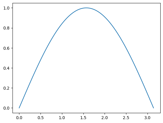
So we don’t have to use awkward list comprehensions when using these.
3.4.5 Multi-Dimensional Arrays#
NumPy’s true power comes from multi-dimensional arrays:
np.zeros([3, 4, 2]) # 3 arrays with 4 rows and 2 columns each
array([[[0., 0.],
        [0., 0.],
        [0., 0.],
        [0., 0.]],

       [[0., 0.],
        [0., 0.],
        [0., 0.],
        [0., 0.]],

       [[0., 0.],
        [0., 0.],
        [0., 0.],
        [0., 0.]]])
Unlike a list-of-lists in Python, we can reshape arrays:
x = np.array(range(40))
x
array([ 0,  1,  2,  3,  4,  5,  6,  7,  8,  9, 10, 11, 12, 13, 14, 15, 16,
       17, 18, 19, 20, 21, 22, 23, 24, 25, 26, 27, 28, 29, 30, 31, 32, 33,
       34, 35, 36, 37, 38, 39])
y = x.reshape([4, 5, 2])  # 4 Arrays - 5 Rows - 2 Columns
y
array([[[ 0,  1],
        [ 2,  3],
        [ 4,  5],
        [ 6,  7],
        [ 8,  9]],

       [[10, 11],
        [12, 13],
        [14, 15],
        [16, 17],
        [18, 19]],

       [[20, 21],
        [22, 23],
        [24, 25],
        [26, 27],
        [28, 29]],

       [[30, 31],
        [32, 33],
        [34, 35],
        [36, 37],
        [38, 39]]])
And index multiple columns at once:
y[3, 2, 1]
35
Including selecting on inner axes while taking all from the outermost:
y[:, 2, 1]
array([ 5, 15, 25, 35])
And subselecting ranges:
y[2:, :1, :] # Last 2 axes, 1st row, all columns
array([[[20, 21]],

       [[30, 31]]])
And transpose arrays:
y.transpose()
array([[[ 0, 10, 20, 30],
        [ 2, 12, 22, 32],
        [ 4, 14, 24, 34],
        [ 6, 16, 26, 36],
        [ 8, 18, 28, 38]],

       [[ 1, 11, 21, 31],
        [ 3, 13, 23, 33],
        [ 5, 15, 25, 35],
        [ 7, 17, 27, 37],
        [ 9, 19, 29, 39]]])
You can get the dimensions of an array with shape
y.shape # 4 Arrays - 5 Rows - 2 Columns
(4, 5, 2)
y.transpose().shape # 2 Arrays - 5 Rows - 4 Columns
(2, 5, 4)
Some numpy functions apply by default to the whole array, but can be chosen to act only on certain axes:
x = np.arange(12).reshape(4, 3)
x
array([[ 0,  1,  2],
       [ 3,  4,  5],
       [ 6,  7,  8],
       [ 9, 10, 11]])
x.mean(1) # Mean along the second axis, leaving the first.
array([ 1., 4., 7., 10.])
x.mean(0) # Mean along the first axis, leaving the second.
array([4.5, 5.5, 6.5])
x.mean() # mean of all axes
5.5
3.4.6 Array Datatypes#
A Python list can contain data of mixed type:
x = ["hello", 2, 3.4]
type(x[2])
float
type(x[1])
int
A NumPy array always contains just one datatype:
np.array(x)
array(['hello', '2', '3.4'], dtype='<U32')
NumPy will choose the least-generic-possible datatype that can contain the data:
y = np.array([2, 3.4])
y
array([2. , 3.4])
You can access the array’s dtype, or check the type of individual elements:
y.dtype
dtype('float64')
type(y[0])
numpy.float64
z = np.array([3, 4, 5])
z
array([3, 4, 5])
type(z[0])
numpy.int64
The results are, when you get to know them, fairly obvious string codes for datatypes: NumPy supports all kinds of datatypes beyond the python basics.
NumPy will convert python type names to dtypes:
x = [2, 3.6, 7.2, 0]
int_array = np.array(x, dtype=int)
int_array
array([2, 3, 7, 0])
int_array.dtype
dtype('int64')
float_array = np.array(x, dtype=float)
float_array
array([2. , 3.6, 7.2, 0. ])
float_array.dtype
dtype('float64')