3.5 Advanced NumPy
Contents
3.5 Advanced NumPy#
Estimated time to complete this notebook: 20 minutes
3.5.1 Recap#
In the previous section we introduced numpy array that represents a multidimensional matrix \(M_{i,j,k...n}\). Which, among other things, allows for vectorised versions of common functions.
import numpy as np
3.5.2 Broadcasting#
This is another really powerful feature of NumPy.
By default, array operations are element-by-element:
np.arange(5) * np.arange(5)
array([ 0, 1, 4, 9, 16])
If we multiply arrays with non-matching shapes we get an error:
np.arange(5) * np.arange(6)
---------------------------------------------------------------------------
ValueError                                Traceback (most recent call last)
Cell In[3], line 1
----> 1 np.arange(5) * np.arange(6)

ValueError: operands could not be broadcast together with shapes (5,) (6,)
np.zeros([2, 3]) * np.zeros([2, 4])
---------------------------------------------------------------------------
ValueError                                Traceback (most recent call last)
Cell In[4], line 1
----> 1 np.zeros([2, 3]) * np.zeros([2, 4])

ValueError: operands could not be broadcast together with shapes (2,3) (2,4)
m1 = np.arange(100).reshape([10, 10])
m2 = np.arange(100).reshape([10, 5, 2])
m1 + m2
---------------------------------------------------------------------------
ValueError                                Traceback (most recent call last)
Cell In[7], line 1
----> 1 m1 + m2

ValueError: operands could not be broadcast together with shapes (10,10) (10,5,2)
Arrays must match in all dimensions in order to be compatible:
np.ones([3, 3]) * np.ones([3, 3]) # Note elementwise multiply, *not* matrix multiply.
array([[1., 1., 1.],
       [1., 1., 1.],
       [1., 1., 1.]])
m3 = np.arange(9).reshape([3, 3])
m3
array([[0, 1, 2],
       [3, 4, 5],
       [6, 7, 8]])
m4 = np.arange(9, 18).reshape([3, 3])
m4
array([[ 9, 10, 11],
       [12, 13, 14],
       [15, 16, 17]])
m3 * m4 # Note elementwise multiply, *not* matrix multiply.
array([[  0,  10,  22],
       [ 36,  52,  70],
       [ 90, 112, 136]])
Except, that if one array has any Dimension 1, then the data is REPEATED to match the other.
col = np.arange(10).reshape([10, 1])
col
array([[0],
       [1],
       [2],
       [3],
       [4],
       [5],
       [6],
       [7],
       [8],
       [9]])
row = col.transpose()
row
array([[0, 1, 2, 3, 4, 5, 6, 7, 8, 9]])
col.shape # "Column Vector"
(10, 1)
row.shape # "Row Vector"
(1, 10)
row + col
array([[ 0,  1,  2,  3,  4,  5,  6,  7,  8,  9],
       [ 1,  2,  3,  4,  5,  6,  7,  8,  9, 10],
       [ 2,  3,  4,  5,  6,  7,  8,  9, 10, 11],
       [ 3,  4,  5,  6,  7,  8,  9, 10, 11, 12],
       [ 4,  5,  6,  7,  8,  9, 10, 11, 12, 13],
       [ 5,  6,  7,  8,  9, 10, 11, 12, 13, 14],
       [ 6,  7,  8,  9, 10, 11, 12, 13, 14, 15],
       [ 7,  8,  9, 10, 11, 12, 13, 14, 15, 16],
       [ 8,  9, 10, 11, 12, 13, 14, 15, 16, 17],
       [ 9, 10, 11, 12, 13, 14, 15, 16, 17, 18]])
10 * row + col
array([[ 0, 10, 20, 30, 40, 50, 60, 70, 80, 90],
       [ 1, 11, 21, 31, 41, 51, 61, 71, 81, 91],
       [ 2, 12, 22, 32, 42, 52, 62, 72, 82, 92],
       [ 3, 13, 23, 33, 43, 53, 63, 73, 83, 93],
       [ 4, 14, 24, 34, 44, 54, 64, 74, 84, 94],
       [ 5, 15, 25, 35, 45, 55, 65, 75, 85, 95],
       [ 6, 16, 26, 36, 46, 56, 66, 76, 86, 96],
       [ 7, 17, 27, 37, 47, 57, 67, 77, 87, 97],
       [ 8, 18, 28, 38, 48, 58, 68, 78, 88, 98],
       [ 9, 19, 29, 39, 49, 59, 69, 79, 89, 99]])
This works for arrays with more than one unit dimension.
3.5.3 Another example#
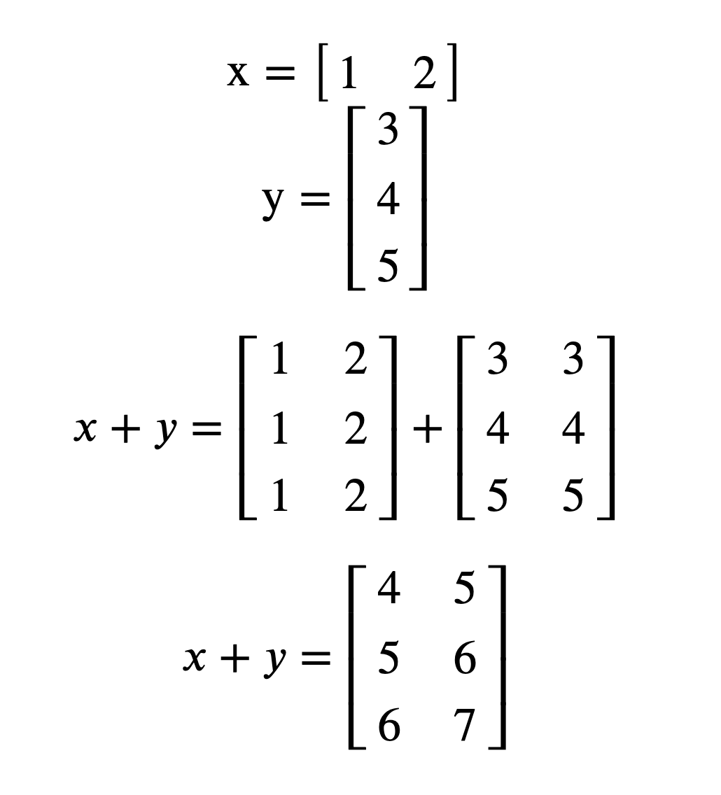
x = np.array([1, 2]).reshape(1, 2)
x
array([[1, 2]])
y = np.array([3, 4, 5]).reshape(3, 1)
y
array([[3],
       [4],
       [5]])
result = x + y
result.shape
(3, 2)
result
array([[4, 5],
       [5, 6],
       [6, 7]])
What numpy is doing:
3.5.4 Newaxis#
Broadcasting is very powerful, and numpy allows indexing with np.newaxis to temporarily create new one-long dimensions on the fly.
import numpy as np

x = np.arange(10).reshape(2, 5)
y = np.arange(8).reshape(2, 2, 2)
x
array([[0, 1, 2, 3, 4],
       [5, 6, 7, 8, 9]])
y
array([[[0, 1],
        [2, 3]],

       [[4, 5],
        [6, 7]]])
x_dash = x[:, :, np.newaxis, np.newaxis]
x_dash.shape
(2, 5, 1, 1)
y_dash = y[:, np.newaxis, :, :]
y_dash.shape
(2, 1, 2, 2)
y_dash
array([[[[0, 1],
         [2, 3]]],


       [[[4, 5],
         [6, 7]]]])
res = x_dash * y_dash
res.shape
(2, 5, 2, 2)
np.sum(res)
830
Note that newaxis works because a \(3 \times 1 \times 3\) array and a \(3 \times 3\) array contain the same data,
differently shaped:
threebythree = np.arange(9).reshape(3, 3)
threebythree
array([[0, 1, 2],
       [3, 4, 5],
       [6, 7, 8]])
threebythree[:, np.newaxis, :]
array([[[0, 1, 2]],

       [[3, 4, 5]],

       [[6, 7, 8]]])
3.5.5 Dot Products using broadcasting#
NumPy multiply is element-by-element, not a dot-product:
a = np.arange(9).reshape(3, 3)
a
array([[0, 1, 2],
       [3, 4, 5],
       [6, 7, 8]])
b = np.arange(3, 12).reshape(3, 3)
b
array([[ 3,  4,  5],
       [ 6,  7,  8],
       [ 9, 10, 11]])
a * b
array([[ 0,  4, 10],
       [18, 28, 40],
       [54, 70, 88]])
We can use what we’ve learned about the algebra of broadcasting and newaxis to get a dot-product, (matrix inner product).
First we add new axes to \(A\) and \(B\):
a[:, :, np.newaxis].shape
(3, 3, 1)
b[np.newaxis, :, :].shape
(1, 3, 3)
Now we use broadcasting to generate \(A_{ij}B_{jk}\) as a 3-d matrix:
a[:, :, np.newaxis] * b[np.newaxis, :, :]
array([[[ 0,  0,  0],
        [ 6,  7,  8],
        [18, 20, 22]],

       [[ 9, 12, 15],
        [24, 28, 32],
        [45, 50, 55]],

       [[18, 24, 30],
        [42, 49, 56],
        [72, 80, 88]]])
Then we sum over the middle, \(j\) axis, [which is the 1-axis of three axes numbered (0,1,2)] of this 3-d matrix. Thus we generate \(\Sigma_j A_{ij}B_{jk}\).
(a[:, :, np.newaxis] * b[np.newaxis, :, :]).sum(1)
array([[ 24,  27,  30],
       [ 78,  90, 102],
       [132, 153, 174]])
Or if you prefer:
(a.reshape(3, 3, 1) * b.reshape(1, 3, 3)).sum(1)
array([[ 24,  27,  30],
       [ 78,  90, 102],
       [132, 153, 174]])
We can see that the broadcasting concept gives us a powerful and efficient way to express many linear algebra operations computationally.
3.5.6 Dot Products using numpy functions#
However, as the dot-product is a common operation, numpy has a built in function:
np.dot(a, b)
array([[ 24,  27,  30],
       [ 78,  90, 102],
       [132, 153, 174]])
This can also be written as:
a.dot(b)
array([[ 24,  27,  30],
       [ 78,  90, 102],
       [132, 153, 174]])
If you are using Python 3.5 or later, a dedicated matrix multiplication operator has been added, allowing you to do the following:
a @ b
array([[ 24,  27,  30],
       [ 78,  90, 102],
       [132, 153, 174]])
3.5.7 Record Arrays#
These are a special array structure designed to match the CSV “Record and Field” model. It’s a very different structure from the normal NumPy array, and different fields can contain different datatypes. We saw this when we looked at CSV files:
x = np.arange(50).reshape([10, 5])
record_x = x.view(
    dtype={"names": ["col1", "col2", "another", "more", "last"], "formats": [int] * 5}
)
record_x
array([[( 0,  1,  2,  3,  4)],
       [( 5,  6,  7,  8,  9)],
       [(10, 11, 12, 13, 14)],
       [(15, 16, 17, 18, 19)],
       [(20, 21, 22, 23, 24)],
       [(25, 26, 27, 28, 29)],
       [(30, 31, 32, 33, 34)],
       [(35, 36, 37, 38, 39)],
       [(40, 41, 42, 43, 44)],
       [(45, 46, 47, 48, 49)]],
      dtype=[('col1', '<i8'), ('col2', '<i8'), ('another', '<i8'), ('more', '<i8'), ('last', '<i8')])
Record arrays can be addressed with field names like they were a dictionary:
record_x["col1"]
array([[ 0],
       [ 5],
       [10],
       [15],
       [20],
       [25],
       [30],
       [35],
       [40],
       [45]])
Indeed we can use these methods when parsing CSV files instead of using Pandas.
3.5.8 Logical arrays, masking, and selection#
Numpy defines operators like == and < to apply to arrays element by element:
x = np.zeros([3, 4])
x
array([[0., 0., 0., 0.],
       [0., 0., 0., 0.],
       [0., 0., 0., 0.]])
y = np.arange(-1, 2)[:, np.newaxis] * np.arange(-2, 2)[np.newaxis, :]
y
array([[ 2,  1,  0, -1],
       [ 0,  0,  0,  0],
       [-2, -1,  0,  1]])
y_is_one = y == 1
y_is_one
array([[False,  True, False, False],
       [False, False, False, False],
       [False, False, False,  True]])
aresame = x == y
aresame
array([[False, False,  True, False],
       [ True,  True,  True,  True],
       [False, False,  True, False]])
A logical array can be used to select elements from an array:
y[np.logical_not(aresame)]
array([ 2, 1, -1, -2, -1, 1])
Although when printed, this comes out as a flat list, if assigned to, the selected elements of the array are changed!
y[aresame] = 5
y
array([[ 2,  1,  5, -1],
       [ 5,  5,  5,  5],
       [-2, -1,  5,  1]])
3.5.9 Numpy memory#
NumPy manages memory differently from lists. Changing an element in a copy of a list does not change the original list.
x = list(range(5))
y = x[:]
y[2] = 0
x
[0, 1, 2, 3, 4]
But in NumPy, changing the copy does change the original array!
x = np.arange(5)
y = x[:]
y[2] = 0
x
array([0, 1, 0, 3, 4])
We must use np.copy to force separate memory.
Otherwise NumPy tries its hardest to make slices be views on data.